This tutorial describes how to use Ansys Forte CFD to simulate combustion for a two-stroke marine engine with intake and exhaust ports. Details on how to use Ansys Forte's automatic mesh generation with sliding interfaces, a requirement for 2-stroke engines, is discussed. The tutorial also demonstrates profile creation and the import and loading of an .stl file to start the simulation from the geometry.
The following sections describe the provided files, time required, prerequisites, and a utility for comparing your generated project file (.ftsim) with the one provided in the tutorial download.
We recommend starting with the Ansys Forte Quick Start Guide , which explains the workflow of the Ansys Forte user interface, before doing this tutorial.
The files for this tutorial are obtained by downloading the
two_stroke.zip file
here
.
Unzip two_stroke.zip to your working folder.
FORTE-2stroke .ftsim: A project file of the completed tutorial, for verification or comparison of your progress in the tutorial set-up. The project file includes all the relevant geometry, chemistry set, and spray profile details.
intake_pressure_profile.csv and exhaust_pressure_profile.csv: Two files of data describing the profile of the time-varying pressure for the intake and exhaust.
time_step_size.csv: Adaptive time-step profile.
output_crank_angles.csv: Profile of crank-angle points for spatially resolved output.
FORTE_2stoke.stl: Geometry file for the 2-stroke engine in this project without the chemistry set, spray profile, and other project details. (Optional)
restart_crank_angles.csv: Profile defining restart points. (Optional)
Nom-VelMag_Vector-Centerline.avi: An animation showing the velocity magnitude and piston motion of the meshed system. (Optional)
The tutorial sample file is provided as a download. You have the opportunity to select the location for the file when you download and uncompress the sample files.
Note: This tutorial is based on a fully configured sample project that contains the tutorial project settings. The description provided here covers the key points of the project set-up but is not intended to explain every parameter setting in the project. The .ftsim file has all custom and default parameters already configured; the text highlights only the significant points of the tutorial.
Forte may be launched in a command line mode to perform certain tasks such as preparing a run for execution, importing project settings from a text file, or various other tasks described in the Forte User's Guide. One of these tools allows exporting a textual representation of the project data to a text file.
Example
forte.sh CLI -project <project_name>.ftsim -export tutorial_settings.txt
Briefly, you can double-check project settings by saving your project and then running the command-line utility to export the settings in your tutorial project (<project_name>.ftsim), and then use the command a second time to export the settings in the provided final version of the tutorial. Compare them with your favorite diff tool, such as DIFFzilla. If all the parameters are in agreement, you have set up the project successfully. If there are differences, you can go back into the tutorial set-up, re-read the tutorial instructions, and change the setting of interest.
In this case, a full 3-D geometry is used to simulate a 2-stroke marine engine, including combustion. The fuel in this engine is gasoline and is direct-injected into the combustion chamber.
The FORTE_2stroke.ftsim project file has been preconfigured with all the information that will be discussed in this section. You do not need to input any values but can just follow along, reading the instructions and viewing the settings in the loaded .ftsim. This chapter nevertheless explains step-by-step the process of setting up the project, as an illustration of the features in the user interface.
Open the project file, FORTE_2stroke.ftsim, from the location where you stored the downloaded tutorial files.
A simple engine configuration is used in this tutorial for demonstration purposes. The details of the configuration and simulation settings are presented here.
Table 9.1: Details of the diesel engine geometry used in this tutorial
| Item | Value | Units |
|---|---|---|
| Cycle type | 2-stoke | |
| Fuel injection system | Direct injection, hollow core | |
| Compression ratio | 12.65 | |
| Bore | 8.58 | cm |
| Stroke | 6.73 | cm |
| Squish | 13.97 | cm |
| Fuel | Gasoline |
The mesh is created using the Automated Mesh Generator in Ansys Forte. The values described in Table 9.1: Details of the diesel engine geometry used in this tutorial can be accessed from the FORTE_2stroke.ftsim project file. If you did not already have a pre-configured geometry, you could import a Fluent Mesh file, STL, KIVA-3V, or CGNS geometry file. Fluent Mesh files are the preferred format for importing geometry because they are guaranteed to be water-tight. The Fluent Mesh file can be created as a surface mesh for the geometry in ANSYS Meshing.
The next sections describe the problem, including how to set up the simulation that is represented in the provided .ftsim file, and some results relating to surfaces, spray, and flame, that you can generate.
In this tutorial, we will import an existing geometry into Ansys Forte and set up the
automatic mesh generation using a global mesh size and adapting the mesh near the valves. To
import the geometry, go to the Workflow tree and click Geometry. This opens the
Geometry icon bar. Click the Import Geometry ![]() icon. In the resulting dialog, drop-down and select Surfaces
from one or more STL files. In the dialog that opens with STL file import
options, accept the defaults.
icon. In the resulting dialog, drop-down and select Surfaces
from one or more STL files. In the dialog that opens with STL file import
options, accept the defaults.
The mesh will be automatically generated during the simulations. When the file browser launches, navigate to the folder Tutorial_2stroke, then select FORTE-2stroke.stl. Note that once you have imported the geometry, there are a number of actions that you can perform on the items in the Geometry node, such as scale, rename, transform, invert normals, or delete geometry elements.
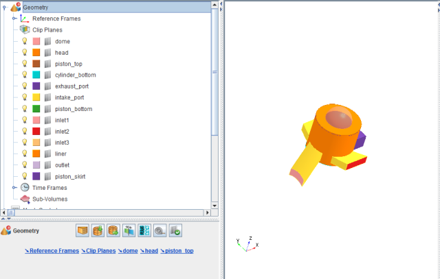
The Geometry imports in an opaque mode and possibly preset zoom level. It is often
helpful to Refit ![]() the view or use the mouse wheel to re-zoom. To change opacity,
right-click the Geometry node in the Workflow tree and select Medium for the Opacity level
of all geometry elements, as shown in Figure 9.2: Two-stroke geometry after import.
the view or use the mouse wheel to re-zoom. To change opacity,
right-click the Geometry node in the Workflow tree and select Medium for the Opacity level
of all geometry elements, as shown in Figure 9.2: Two-stroke geometry after import.
Material Point: On this panel, we must set the point that defines where Ansys Forte will mesh. This point, the Material Point, must always lie inside the geometry during the entire cycle and should be located at least one unit cell length away from any boundaries. On the Material Point Editor panel, define the point’s location as X = 0.0, Y = 0.0, Z = 6.9 cm.
Global Mesh Size: Set the Global Mesh Size to 2.0 mm. Other Mesh Controls should be set to these values:
Table 9.2: Settings for Mesh Control refinements
| Item | Refinement type | Refinement location | Refinement level | Refinement layers | Crank angle active range |
|---|---|---|---|---|---|
| AllSurfaces | Surface Refinement | All walls except inlets and outlet | 1/2 | 1 layer | |
| OpenBoundaries | Surface Refinement | Inlets and Outlet | 1/2 | 12 layers | |
| TDC | Surface Refinement | Head and Piston Top | 1/4 | 2 layers | 350° - 370° |
| PortWalls2 | Surface Refinement | Intake and Exhaust Port | 1/2 | 7 | |
| Combustion | Point |
(0.0, 0.0, 6.0) cm Radius of 4.4 cm | 1/2 | 274° - 400° | |
| Coarse Feature | Feature |
Feature angle =60° Feature Radius of Influence =7.0 mm Intake/Exhaust Port, Liner, Piston Skirt, Piston Top | 1/2 | ||
| Fine Feature | Feature |
Feature angle =60° Feature Radius of Influence =2.0 mm Liner, Piston Skirt, Piston Top | 1/4 | ||
| SAM-G-kernel | SAM using solution field G Bounds = Absolute Range with bounds of -0.3, 0.3 | Entire domain | 1/8 | 319° - 330° | |
| SAM-G | SAM using solution field G Bounds = Absolute Range with bounds of -0.3, 0.3 | Entire domain | 1/4 | 315° - 400° |
Chemistry: Now that the mesh has been set up, assigning models is
next. Assign the chemistry using Models ¬ Chemistry/Materials and use the New
Import Chemistry ![]() icon and select the file
Gasoline_1comp_49sp.cks from the Ansys Forte data
directory. If you are curious, you can view the chemistry details, such as chemistry source,
pre-processing log, gas phase input, gas phase output, thermodynamic input, transport input,
and transport output.
icon and select the file
Gasoline_1comp_49sp.cks from the Ansys Forte data
directory. If you are curious, you can view the chemistry details, such as chemistry source,
pre-processing log, gas phase input, gas phase output, thermodynamic input, transport input,
and transport output.
Flame Speed Model: On the Workflow tree, use Models ¬ Chemistry/Materials ¬ Chemkin Chemistry Set ¬ Flame Speed Model and select the Table Library Option in the Laminar Flame Speed drop-down menu. For Flamespeed Library, select Create new..., then add ic8h18 as the fuel species and specify iso_octane as the name. Click Save and close the Library Editor panel. For the Turbulent Flame Speed settings, keep the defaults. For Unburned Calculation Method, use the Volume Search with Variable Radius option. Click Apply.
The default values are used in the Transport property panel. In the Transport ¬ Turbulence panel, the RNG k-epsilon model is used, with default values.
Models ¬ Spray Model: Since this is a direct-injection case, turn ON (check) Spray Model in the Workflow tree to display its icon bar (action bar) in the Editor panel. In the panel, keep the defaults. Leave the Use Vaporization Model (default) check ON.
Add an Injector: This Icon bar provides multiple spray-injector options. For this
injector, click the Hollow Cone
![]() icon. In the dialog that opens, name the new hollow-cone injector as
Hollow Cone Injector. This opens another icon bar and Editor panel
for the new hollow-cone injector. In the Workflow tree under the Hollow Cone Injector node,
add a Nozzle and an Injection. You can either right-click the Hollow Cone Injector node and
select Add or select that Workflow tree item or use the icons in the
panel’s action bar.
icon. In the dialog that opens, name the new hollow-cone injector as
Hollow Cone Injector. This opens another icon bar and Editor panel
for the new hollow-cone injector. In the Workflow tree under the Hollow Cone Injector node,
add a Nozzle and an Injection. You can either right-click the Hollow Cone Injector node and
select Add or select that Workflow tree item or use the icons in the
panel’s action bar.
On the Hollow Cone Injector panel, create a new Composition, select ic8h18 (iso-octane) in the Species list, specify the physical properties as iso-octane, and specify the Mass Fraction as 1.0. Use iso-octane for the Vaporization properties and name the Composition gasoline. Click Save.
For the injection, specify the following parameters:
Table 9.3: Injection settings used in this tutorial
| Input | Value | Units |
|---|---|---|
| Injected Parcel Count | 30,000 | - |
| Inflow Droplet Temperature | 363 | K |
| Injection Pressure | 51.7 | bar |
| Inwardly Opening Nozzle | Checked (ON) | - |
| Mean Cone Angle | 54.0 | degrees |
| Liquid Jet Thickness | 15.0 | degrees |
| Droplet Size Distribution | Rosin-Rammler Distribution | - |
| Shape Parameter | 3.5 | - |
| Breakup Length Model Constant | 12.0 | - |
With the Hollow Cone Injector selected, add a Nozzle to the injector by clicking the
New Nozzle
![]() icon. On the Nozzle Editor panel, set the parameters as described in
Table 9.4: Nozzle settings used in this tutorial. Click Apply. You
can see the nozzle appear at the top of the geometry. (You may want to make the Geometry
non-opaque or change the color of the nozzle itself by right-clicking in the Workflow tree
and selecting Color or Opacity to make the nozzle
easier to see in the interior.)
icon. On the Nozzle Editor panel, set the parameters as described in
Table 9.4: Nozzle settings used in this tutorial. Click Apply. You
can see the nozzle appear at the top of the geometry. (You may want to make the Geometry
non-opaque or change the color of the nozzle itself by right-clicking in the Workflow tree
and selecting Color or Opacity to make the nozzle
easier to see in the interior.)
Table 9.4: Nozzle settings used in this tutorial
| Location | |
| Reference Frame | Global origin |
| Coordinate system | Cartesian |
| X | 0.0 cm |
| Y | 0.0 cm |
| Z | 9.221 cm |
| Spray Direction | |
| Reference Frame | Global origin |
| Coordinate System | Spherical |
| Θ | 180 degrees |
| Φ | 0.0 degrees |
| Nozzle Size | |
| Nozzle Area | 0.001647 cm2 |
Injection: On the Injection panel, specify the Start of Injection as 275 degrees, the Duration of Injection as 12.42 degrees, specify the Velocity Profile as a Square Profile, and the Injected Mass as 0.007292 g.
Spark Ignition: Turn on the spark ignition model by checking the box at Models ¬ Spark Ignition. Keep the defaults for the Spark Ignition settings except Kernel Flame to G-equation Switch Constant = 2.0.
Use the New Spark
 icon to create a new spark event and name it
Spark.
icon to create a new spark event and name it
Spark.
Use Models ¬ Spark Ignition ¬ Spark to set up the details of the spark event. In the Location, for Reference Frame, use Global Origin and Cartesian coordinates for the Location, and set X = 1.233 cm, Y = 0.0 cm, and Z = 7.76 cm. Select Crank Angle for Timing Option and Starting Angle = 319.0 degrees, Duration = 9.0 degrees. Under Spark Energy, set Energy Release Rate = 25.0 J/sec. Accept the default 0.5 for Energy Transfer Efficiency and 0.5 mm (note that the unit is mm) for Initial Kernel Radius. Click Apply.
Boundary conditions specify inlets, outlets, and walls. Once you create one boundary
condition, you can copy and paste it (using the Copy
![]() and Paste
and Paste
![]() icons on the icon bar in the Editor panel), then modify it to create a
second boundary condition. Select a boundary surface, either from the list in the workflow
tree or using the Select from Screen
icons on the icon bar in the Editor panel), then modify it to create a
second boundary condition. Select a boundary surface, either from the list in the workflow
tree or using the Select from Screen
![]() tool to pick a surface in the 3-D View to associate with a boundary
condition.
tool to pick a surface in the 3-D View to associate with a boundary
condition.
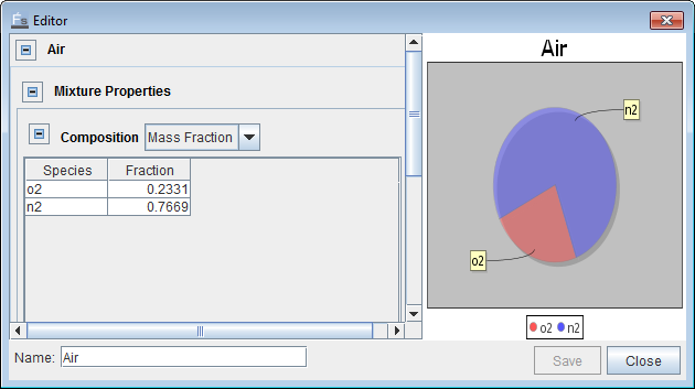
Inlet: From the Boundary Conditions node, in the Editor panel,
click the New Inlet  icon and create an Inlet named Inlet1. At the top
of the Editor panel, select Create new gas mixture... for the
Composition. Click the Add Species button and then select
o2 (oxygen) and n2 (nitrogen) as the species.
Specify Mass Fraction of 0.23 for
o2 and 0.77 for n2, as shown
in Figure 9.3: Composition editor specifying inlet Air mixture. Name the composition
Air and click Save then
Close.
icon and create an Inlet named Inlet1. At the top
of the Editor panel, select Create new gas mixture... for the
Composition. Click the Add Species button and then select
o2 (oxygen) and n2 (nitrogen) as the species.
Specify Mass Fraction of 0.23 for
o2 and 0.77 for n2, as shown
in Figure 9.3: Composition editor specifying inlet Air mixture. Name the composition
Air and click Save then
Close.
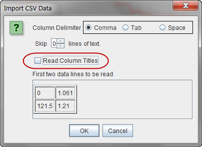
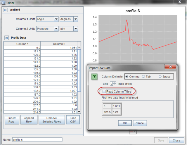
In the Editor panel, select inlet1 from the Location list. Select Total Pressure, Time Varying as the Inlet Option. Select Crank Angle in the Time Option drop-down menu and for the pressure profile, select Create new... and import the pressure profile using the Load CSV option. The name of the pressure profile is intake_pressure_profile.csv. On the Load CSV dialog, clear (deselect) the Read Column Titles option (because the file does not contain any column titles), as shown in Figure 9.4: Import CSV data for pressure profile. The unit for Column 1 should be Angle and degrees and for Column 2 the units should be Pressure and bar.
The pressure profile should look like the profile shown in Figure 9.5: Importing the intake pressure profile.
Define Turbulence using values for Turbulent Kinetic Energy and Length Scale of 3,600 cm2/sec2 and 1.0 cm, respectively. On the Editor panel, accept Assume Isentropic for the Temperature Option. Click Apply.
Now that the first inlet has been created, copy and paste inlet1
and name it inlet2 using the Copy
![]() and Paste.
and Paste. ![]() icons. Repeat this step to create inlet3. Update
the Location to inlet2 and inlet3, respectively,
for each new boundary condition, inlet2 and
inlet3.
icons. Repeat this step to create inlet3. Update
the Location to inlet2 and inlet3, respectively,
for each new boundary condition, inlet2 and
inlet3.
Outlet: From the Boundary Conditions node, go to the Editor panel
and click the New Outlet  icon and create Outlet. I the Editor panel,
select outlet from the Location list. Select
Total Pressure, Time Varying as the Outlet Option.
For the pressure profile, select Create New and import the pressure
profile using the Load CSV option. The name of the pressure profile is
exhaust_pressure_profile.csv. On the Load CSV dialog, deselect the
Read Column Titles option, because the file does not contain any column
titles. The unit for Column 1 should be Angle and
degrees, and for Column 2 the units should be
Pressure and bar. Set the Turbulence
Boundary Conditions to Turbulent Kinetic Energy and Length
Scale of 3,600 cm2/sec2 and 1.0 cm,
respectively.
icon and create Outlet. I the Editor panel,
select outlet from the Location list. Select
Total Pressure, Time Varying as the Outlet Option.
For the pressure profile, select Create New and import the pressure
profile using the Load CSV option. The name of the pressure profile is
exhaust_pressure_profile.csv. On the Load CSV dialog, deselect the
Read Column Titles option, because the file does not contain any column
titles. The unit for Column 1 should be Angle and
degrees, and for Column 2 the units should be
Pressure and bar. Set the Turbulence
Boundary Conditions to Turbulent Kinetic Energy and Length
Scale of 3,600 cm2/sec2 and 1.0 cm,
respectively.
Piston: From the Boundary Conditions node, go to the Editor panel
and click the New Wall  icon and name it Piston_Moving. Select the
piston_top item in the Location list. Set the
Thermal Boundary Condition to Wakk Temperature,
Constant and 450 K. Turn ON the
Wall Motion option and set the piston Motion Type
to use a Slider Crank with a Stroke of
6.73 cm and a Connecting Rod Length of
13.97 cm with 0.0 cm Piston Offset. To set the
axis for translation, under Direction, the Reference
Frame is Global Origin and the Coordinate
System is Cartesian. Set X = 0.0 cm, Y = 0.0 cm, Z
= 1.0 cm. Change the Movement Type to Sliding
Interface and select the liner and
piston_skirt from the list of surfaces. For this setting, the moving
piston should be selected along with the surface it is sliding/moving past.
icon and name it Piston_Moving. Select the
piston_top item in the Location list. Set the
Thermal Boundary Condition to Wakk Temperature,
Constant and 450 K. Turn ON the
Wall Motion option and set the piston Motion Type
to use a Slider Crank with a Stroke of
6.73 cm and a Connecting Rod Length of
13.97 cm with 0.0 cm Piston Offset. To set the
axis for translation, under Direction, the Reference
Frame is Global Origin and the Coordinate
System is Cartesian. Set X = 0.0 cm, Y = 0.0 cm, Z
= 1.0 cm. Change the Movement Type to Sliding
Interface and select the liner and
piston_skirt from the list of surfaces. For this setting, the moving
piston should be selected along with the surface it is sliding/moving past.
Note: The RPM is specified on the Simulation Controls Editor panel.
Intake: Click the New Wall
icon and name it IntakePort. Select the
intake_port item in the Location list and turn
ON the Heat Transfer option and set the
Temperature to 300 K.
Now reproduce the Intake Port with Copy
![]() and Paste
and Paste
![]() four times to create four new boundaries as detailed in the following
table.
four times to create four new boundaries as detailed in the following
table.
Table 9.5: Details of boundaries created from Copy and Paste operations
| Item | Boundary Name | Location | Boundary Condition |
|---|---|---|---|
| 1 | ExhaustPort | exhaust_port |
Wall Model=Law of the Wall Twall=490 K Heat Transfer=ON |
| 2 | Liner |
cylinder_bottom liner |
Wall Model=Law of the Wall Twall=400 K Heat Transfer=ON |
| 3 | Head |
dome head |
Wall Model=Law of the Wall Twall=400 K Heat Transfer=ON |
| 4 | Piston_Anchored |
piston_bottom piston_skirt |
Wall Model=Law of the Wall Twall=450 K Heat Transfer=ON |
The domain is initialized with the operating conditions, species concentrations and temperatures. The Default Initialization species composition is at the expected exhaust composition, assuming complete combustion. The intake and exhaust must also be initialized to the boundary condition values. Set the initialization parameters as described in the following sections.
Initialization Order: When looking at the piston in the TDC position, each isolated region should have an initialization region with a material point specified, which is typically the combustion chamber, the exhaust port, and the intake port. In many cases, there will be multiple intake regions that will require their own initialization, as in this case.
For 2-stroke engine cases, the combustion chamber should have an initialization order of 1. The intake ports should then have initialization orders of 2, 3, and 4, respectively. Lastly, the exhaust port would have an initialization order of 5.
Default Initialization:
Select Default Initialization in the Workflow tree. In the Editor panel, set the Initialization Order to 1. (For 2-stroke engines, the combustion chamber should have an Initialization Order of 1.) Select Create new gas mixture... in the Composition drop-down list and click the Pencil
 icon. This opens the Gas Mixture panel, where you select
Add Species. Set a Mass Fraction of
o2=0.1123911, n2=0.7421674,
co2=0.0996009, and h2o=0.0458404, and
Save this composition as Exhaust_Est. On the
Editor panel, set a Constant Temperature of 1,220
K and a Constant Pressure of 2.7
bar.
icon. This opens the Gas Mixture panel, where you select
Add Species. Set a Mass Fraction of
o2=0.1123911, n2=0.7421674,
co2=0.0996009, and h2o=0.0458404, and
Save this composition as Exhaust_Est. On the
Editor panel, set a Constant Temperature of 1,220
K and a Constant Pressure of 2.7
bar. The Turbulence initialization uses the Constant option and the Turbulent Kinetic Energy and Length Scale option with values 3,600 cm2/sec2 and 1.0 cm, respectively.
The Velocity is initialized by using Constant Velocity and selecting Velocity Components and accepting defaults.
Click Apply.
Intake Initialization: The intake Initial Condition is set to match the Boundary Condition at the Inlet. Since this is a separate port that can be closed off from the main cylinder region, we also need to set the equivalent of a material point to identify the region, as well as an initialization order that helps determine what region takes precedence in initializing new cells that appear when gaps are opened.
From the Initial Conditions Editor panel, select the New Secondary Region From Material Point
 icon and name it Intake1.
To identify the region, select a point for the Location under the Reference Frame = Global Origin selection, which is a point that will always be within the Intake1 port. Set the Cartesian and the coordinates to X = 0.0, Y = 6.0, Z = 1.2 cm, which is a point just inside the inlet.
Set the Initialization Order to 2. Initialization order follows flow order.
Set the Composition by selecting in the previously saved profile, Air. Set the Temperature to Constant and 300 K and Pressure to Constant and 1.013 bar. The Turbulence initialization is Constant and uses the Turbulent Kinetic Energy and Length Scale option set to 3,600 cm2/sec2 and 1.0 cm, respectively. The Velocity is initialized by using Constant Velocity and Velocity Components and accepting defaults. Click Apply.
Copy
 and Paste
 Intake1 twice, naming the new initializations
Intake2 and Intake3. All the settings are
the same, except for the Initialization Order and
Location:
Intake1 twice, naming the new initializations
Intake2 and Intake3. All the settings are
the same, except for the Initialization Order and
Location:Intake # Coordinates Initialization Order Intake2 X = -4.8, Y = 0.0, Z = -1.0 cm 3 Intake3 X = 0.0, Y = -5.0, Z = 1.2 cm 4
Exhaust Initialization: The Initial Conditions of the Exhaust are set to match the Boundary Condition of the Outlet.
From the Initial Conditions panel, select the New Secondary Region from Material Point
icon and name it ExhaustPort.To identify the region, select a point for the Location under the Reference Frame selection, which is a point that will always be within the ExhaustPort region. Set the coordinates for this case to X = 6.0, Y = 0.0, Z = 1.4 cm.
Set the Initialization Order to 5. Flow is expected to go from the cylinder to the exhaust port; for this reason, we give it the last order in initialization precedence for the 5 regions defined.
Set the Composition to Constant and the existing profile, Exhaust_Est. Set the Temperature to 490 K and Pressure to a Constant 0.981 bar.
The Turbulence initialization uses a Constant Turbulent Kinetic Energy and Length Scale option; these are set to 3,600 cm2/sec2 and 1.0 cm, respectively.
The Velocity is initialized using Constant Velocity and selecting Velocity Components and accepting defaults. Click Apply.
Simulation controls allow you to define the simulation limits, RPM, time step, chemistry solver, and transport terms.
Simulation Limits: Ansys Forte uses adaptive time stepping, with user-specified initial time step and maximum time step. Use Crank Angle Based limits, the simulation Start Crank Angle (that is, Initial Crank Angle, under Simulation Controls in the Workflow tree) is set to 97.0 degrees ATDC, and the simulation Final Simulation Crank Angle is set to 455.0 degrees ATDC. Set RPM to 2,000 rpm and Cycle Type to 2-Stroke.
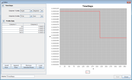
Time Step: Ansys Forte uses adaptive time stepping, with user-specified initial time step and maximum time step. Use Simulation Controls ¬ Time Step and accept the defaults except:
Set the Max. Time Step Option to Crank Angle Based Profile and set up a profile to control the variation in time steps. This allows the maximum time step to be reduced at times of high interest, such as the spark and injection, and decreased during other intervals. In the drop-down list for Max Time Step Profile, select Create new... and click the Pencil
 icon. Because this is a 2-stroke engine, the simulation should run
from 0 to 360 CA degrees. After setting the
following parameters, click Save.
icon. Because this is a 2-stroke engine, the simulation should run
from 0 to 360 CA degrees. After setting the
following parameters, click Save.
| Column 1 | Column 2 |
|---|---|
| Units = Angle and degrees | Units = Time and sec |
| 0.0 | 1.00E-5 |
| 215.0 | 1.00E-5 |
| 216.0 | 5.00E-6 |
| 360.0 | 5.00E-6 |
| Name of profile: TimeSteps | |
The Editor panel for creating the profile will resemble Figure 9.6: TimeSteps profile for Max Time Step Profile.
Chemistry Solver: Simulation Controls ¬ Chemistry Solver is also kept at the defaults for the following solver tolerances:
Do not activate Dynamic Adaptive Chemistry. DAC should not be used for this case since there are fewer than 500 species. For cases with 500+ species, DAC may provide additional speedup in the simulation.
Use Dynamic Cell Clustering to take advantage of groups of cells with similar conditions. Select 2 features to introduce Dynamic Cell Clustering: 1) Max. Temperature Dispersion of 10 K and 2) a Max. Equilibrium Ratio Dispersion of 0.05.
To increase the time-to-solution speed, you have the ability to choose when chemistry is activated. In this tutorial, select Activate Chemistry Conditionally, turn ON (check) After Fuel Injection Starts, and select When Temperature is Reached with Threshold Temperature = 600 K. This ensures that chemistry is active during the time that combustion is expected. Click Apply.
Output controls determine what data are stored for viewing during the simulation and for creating plots, graphs, and animations in Ansys Forte Visualize, CFD-Post, or EnSight.
The following species are named in both the Spatially Resolved and Spatially Averaged and Spray Output Control Editor panels, to be written to the results file. Fuel, oxidizer, and common emissions species are automatically added. Move these species into the Selection list.
n2
o2
co2
h2o
co
no
no2
ic8h18
The spatially resolved values are output at intervals of 20 crank angles, and the spatially averaged values every 1.0 crank angle. On each of the panels, click Apply.
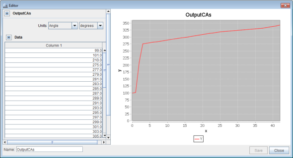
Output Controls ¬ Spatially Resolved: On this Editor panel, you can also optionally increase the frequency of output during the cycle by selecting User Defined Output Control and importing the output_crank_angles.csv file, which has a list of specific crank angles where spatially resolved output will occur. Specify the name of the profile as output _crank_angles. Alternatively, you could select User Defined Output Control, and use the Profile Editor to create the same profile, or some other file specifying an output crank-angle profile (the provided profile is illustrated in Figure 9.7: Output CAs profile for Spatially Resolved output ). Click Save once the profile is imported and the name is specified.
Output Controls ¬ Spatially Averaged: This Editor panel allows you to control the output of values that are averaged across the domain. Keep the default species and solution variables selected for output. Reducing the variables selected will help reduce file sizes.
Restart Data: If you anticipate that the case will be stopped and you want the ability to restart it from the last time step solved, select Output Controls ¬ Restart Data. You can specify certain Restart Points using a separate file. Turn ON (checkmark) User Defined Restart Points and use the Profile Editor to create a Restart profile. You can view, edit, or import new Restart Points in this 1-D Profile Editor. Sometimes it is helpful in spark ignition cases to save a restart file after IVC but before the spark occurs (CA=319 in this case) so you can use the compression portion of the cycle as a start point in additional runs. Create a new profile for this purpose called Restart_crank_angles and add the lines with CA value set to 274.0, 318.0, 400.0 CA degrees. Click Save.
You can view the profiles for accurate boundary motion and appropriate mesh quality with the Preview Simulation options.
Boundary Motion: Preview boundary motion with the player buttons on the Boundary Motion Editor panel or by right-clicking the Boundary Motion item in the Workflow tree and selecting a command. During the preview, a dotted line tracker provides a representation of the piston translation and the location of the injection and spark events (in the Editor panel), and the piston’s motion (in the 3-D View if visibility settings are appropriate).
Preview Mesh: As a method for checking the automatically generated mesh, you can generate a Preview Mesh. Navigate to Preview Simulation ¬ Mesh Generation on the Workflow tree. The preview data will be transferred to a new EnSight instance where it can be viewed with the full suite of EnSight tools.
Select Crank Angle as the Time Option and enter 98.0 degrees, representing the start of the simulation. Enter Start as the Data Set Name.
Select Save Output to Disk to have the preview data persist on disk for loading later into EnSight. If Save Output to Disk is not selected, the preview will run in runtime memory only and will be discarded once the EnSight session is closed.
Select Include Volume Mesh to indicate that the interior volume mesh should be generated. If Include Volume Mesh is not selected, the preview data will only include surface mesh data.
For MPI Arguments, enter the number of MPI processes to be used to generate the preview data.
Once the changes have been applied, click the  button on the Editor panel's toolbar. If Save Output to
Disk is selected, the mesh generation will run in the background, and when
complete, pressing the EnSight button will initiate a session. If Save Output to
Disk is not selected, an EnSight instance is launched immediately.
button on the Editor panel's toolbar. If Save Output to
Disk is selected, the mesh generation will run in the background, and when
complete, pressing the EnSight button will initiate a session. If Save Output to
Disk is not selected, an EnSight instance is launched immediately.
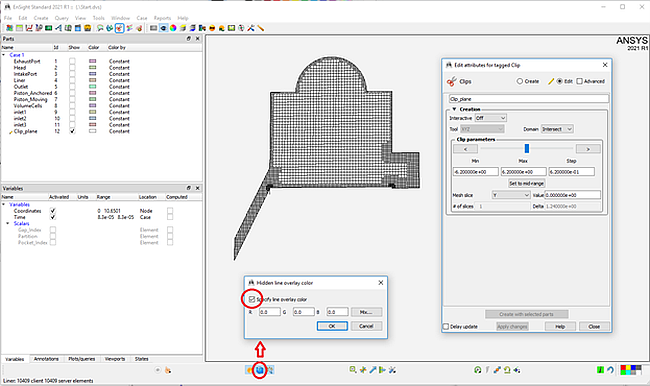
A common workflow for evaluating the preview mesh within the EnSight application is:
Create a clip plane from the VolumeCells part. In this case, select a Y-Clip at Mid-range, as indicated in Figure 9.8: Preview mesh in EnSight at 98 CA degrees, the start of the simulation.
Toggle the VolumeCells part and all of the surface parts’ visibility to OFF.
Turn on mesh lines as shown in Figure 9.8: Preview mesh in EnSight at 98 CA degrees, the start of the simulation by enabling a Hidden Line Overlay Color.
You can create and save additional data sets to disk by supplying a different data set name and altering the time or crank angle value. Additionally, multiple meshes can be generated at the same time using the Time Range or Angle Range options.
The settings here depend on the system and environment for your simulations. The default for the Run Settings panel is to have nothing selected.
Run Options: This tutorial does not require changes to this panel’s defaults; adjust them as necessary for your environment.
Windows Settings: This tutorial does not require changes to this panel’s defaults; adjust them as necessary for your environment.
Linux Settings: This tutorial does not require changes to this panel’s defaults; adjust them as necessary for your environment.
The last step is to submit the simulation to the solver or prepare for submission on a cluster.
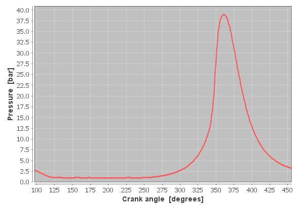
To complete the lesson, select Run Simulation on the Workflow tree and click the blue
arrow Start button. You can monitor the results by clicking on the
Monitor Runs  icon. In the Monitor window that opens, you can select the run you want
to monitor. The pressure trace should look like the one in Figure 9.9: Monitoring the pressure from Run Simulation. This simulation takes about 11 hours to complete on
20 cores (Intel® Xeon® E5-2690 @2.9GHz).
icon. In the Monitor window that opens, you can select the run you want
to monitor. The pressure trace should look like the one in Figure 9.9: Monitoring the pressure from Run Simulation. This simulation takes about 11 hours to complete on
20 cores (Intel® Xeon® E5-2690 @2.9GHz).
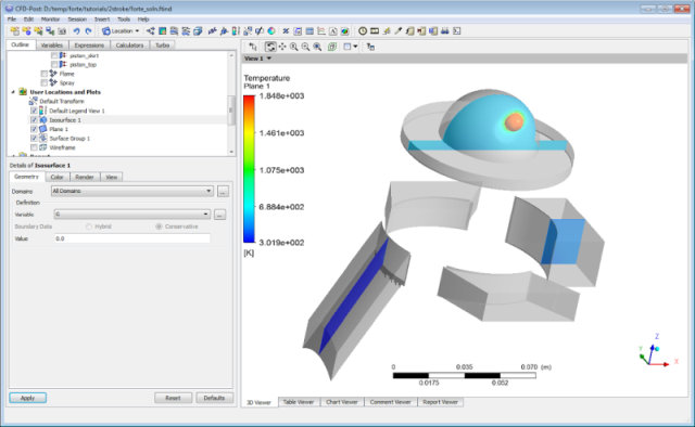
To view the results of the simulation, open the results in CFD-Post. In CFD-Post, open the solution file for the case (Nominal.ftind). Figure 9.10: Screen view of the solution file in CFD-Post shows the screen view once the solution file has been loaded.
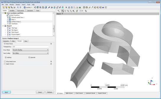
Once you have read in the model, you can create surface groups to group the surfaces. In this case, we will create a surface group for the spark plug, walls, symmetry boundaries, and the valves. To create a surface group, right-click User Locations and Plots Insert > Locations > Surface Group and specify the name surfaces. On the Color and Render tab, you can change the color of the surfaces and the transparency. In Figure 9.10: Screen view of the solution file in CFD-Post, the surfaces are colored gray and the transparency is set to a value of 0.5.
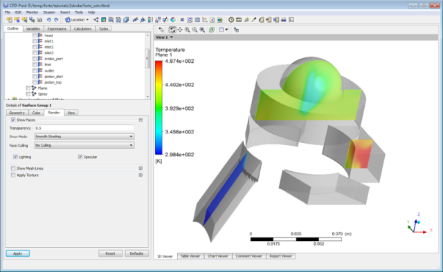
To visualize the solution in the combustion chamber, create a cut plane by right-clicking User Locations and Plots > Insert > Location > Plane. Specify the Method as a ZX plane. On the Color tab, set the Mode to Variable and specify the Variable as Temperature, click Apply. The temperature is now displayed on the cut plane, as shown in Figure 9.11: Temperature contour plot on a plane through the centerline of the combustion chamber.
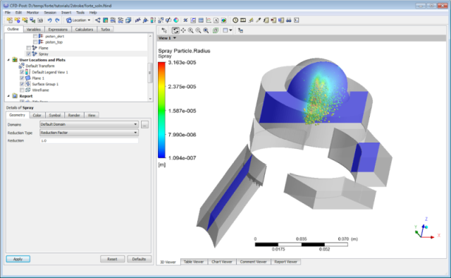
To visualize the spray injection into the chamber, activate the Spray option. Double-click Spray to edit the settings. On the Color tab, set Mode to Variable and select Spray Particle Radius. Set the Range to Local. To visualize the spray at a specific crank angle, go to Tools > Timestep Selector. In this case, crank angle 291.02 is specified.
Finally, to visualize the position of the flame, we need to create an iso-surface. To create the iso-surface, right-click User Locations and Plots and select Insert > Location > Isosurface. Specify flame as the name of the surface. Specify G as the variable and specify red as the color for the surface on the Color tab. To see the flame location, we must specify a crank angle after spark timing. Spark timing in this case is 319 CA degrees, so you can use the menu command Tools > Timestep Selector to select a crank angle after spark timing.