


The Chemistry/Materials node is used to specify the working fluid's compositions, thermodynamics data, and chemical reactions, using the industry-standard Ansys Chemkin format. It also provides settings for the thermodynamic Equation of State, and phase change, if applicable. Click Models > Chemistry/Materials to open its panel.
In Ansys Forte 2022 R1, "Materials" was added to the "Chemistry" model node of the Workflow tree, and new nodes have been added below this node.
This node of the Workflow tree is described in the following sections.
Ansys Forte simulation needs a Chemkin chemistry set file (.cks) to
determine which chemical species or molecules are available in the simulation, their
thermodynamic data, and the available chemical reactions. On the Chemistry/Materials
panel, the View Chemistry  icon in the icon bar lets you view the chemistry set that has been loaded
into your Forte project. If there is no chemistry set in the project, as is the case in any
new project, you have three options to provide it:
icon in the icon bar lets you view the chemistry set that has been loaded
into your Forte project. If there is no chemistry set in the project, as is the case in any
new project, you have three options to provide it:
(1) Click the New Import Chemistry  icon to import a pre-defined chemistry set file. This opens a file browser
to select and load the chemistry set file (.cks). You can navigate to the
data directory of your Ansys Forte installation location and find a number of
chemistry set files that come with the installation, which are created for different types of
simulation problems. Alternatively, you can load a self-made chemistry set file at any other
location.
icon to import a pre-defined chemistry set file. This opens a file browser
to select and load the chemistry set file (.cks). You can navigate to the
data directory of your Ansys Forte installation location and find a number of
chemistry set files that come with the installation, which are created for different types of
simulation problems. Alternatively, you can load a self-made chemistry set file at any other
location.
(2) Use the Chemistry Set Pre-Processing
Utility to create a chemistry set file. The menu (on the
main toolbar) provides the Pre-Processing Utility to create such a chemistry set file from more
fundamental Chemkin input files, including the reaction-mechanism input and the thermodynamic
data file. This utility is described in Chemistry Set Pre-Processing Utility. After the chemistry set file is
created and saved, click the New Import Chemistry icon to import it from the chemistry set from its saved location.
Tip: These two options are commonly used to set up a gas phase flow simulation with combustion processes. Inclusion of chemical reactions in the chemistry set is necessary for reacting flow simulations.
After a chemistry set is imported, a Chemkin Chemistry Set node
appears under Chemistry/Materials. There are three icons on its panel. The
Import Chemistry icon allows you to import a chemistry set file to override the existing
one. The View Chemistry icon opens a panel displaying details associated with the imported
chemistry set. The information shown in the Gas Phase Output tab is particularly helpful as it
lists the chemical species and reactions specified. Reload Chemistry  is similar to Import Chemistry , but it starts the import process using the existing chemistry set file if
it exists in the project.
is similar to Import Chemistry , but it starts the import process using the existing chemistry set file if
it exists in the project.
(3) The third option to add a chemistry set is to click the New Liquid & Vapor Pair and/or the New Gas Species icons on the Chemistry/Materials panel. This option is used to automatically generate a chemistry set file in the Forte project based on user-selected fluid species. Use New Liquid & Vapor Pair to add both liquid and vapor of a specific chemical species. Use New Gas Species to add a specific gas species. You can add multiple liquid and vapor pairs and/or gas species, and the chemistry set is generated by incorporating all the species. However, the chemistry set does not include any chemical reaction. Therefore, use of this option is suitable for non-reacting flow simulation.
When you View Chemistry, the added gas species are listed in the Gas Phase Output, and the added liquid species are listed in the Surface Output. Presence of liquid species is necessary if the simulation is Eulerian two-phase (described next), which requires specifying a multiphase mixture (see Mixture Editor) as the working fluid.
By default, the property data of the liquid species come from an internal library of Ansys Forte. You may choose to override certain liquid properties from the library using your own data. To do so for a specific liquid, click to select the liquid and vapor pair, select User Defined Values for Liquid Properties, check Override Database Liquid Density/Viscosity/Vapor Pressure/Specific Heat/Heat Vaporization/Conductivity/Surface Tension with Constant Value, and fill in the desired data.
Note: Two properties listed on that panel - and , are not used by the Forte solver at this time. Overriding these properties will not change the simulation results.
On the Chemistry/Materials panel, you can select the Equation of State options under Global Gas Phase Settings. These options allow specifying a thermodynamic Equation of State for the gas phase working fluid, which is used together with conservation laws as governing equations for the fluid flow. The three available options are: Ideal Gas, Real Gas, and Use RGP File (Real Gas Property table file). By default, the Ideal Gas law is applied because it is the simplest and most-used relation.
You may select the Real Gas model, which uses cubic Equation of State
to model the gas’ thermodynamic relations. This model is helpful in situations where
gases do not follow the assumptions of ideal gas, such as high-pressure and low-temperature
conditions. The real gas model is dependent on several parameters that are specific to
individual gas species, namely, critical temperature, critical pressure, critical specific
volume, and acentric factor. Therefore, the real gas model is only applicable if the imported
chemistry set contains real-gas-related property data for the defined working fluid. To check
if the real gas data are contained in the chemistry set, click View
Chemistry , and look for Real Gas Information in the Gas Phase
Output tab. If it is present, the species with real gas data available are listed in the lower
area of the tab.
Tip: Most chemistry sets in the data directory of your Ansys Forte
installation location contain real gas data. If your chemistry set does not contain real gas
data, they need to be added in the gas phase kinetics input file
(chem.inp). For more details on the required data format, refer to Real Gas Data in the Chemkin Input Manual. After the input file is
ready, use the Chemistry Set Pre-Processing Utility to create a new
chemistry set file, import it into the Forte project, and View
Chemistry to verify that the real gas data are successfully added.
If the Use RGP File option is selected, the thermodynamic relations are obtained from the Real Gas Property (RGP) Table rather than modeling equations. An RGP file name must be provided when the corresponding option is chosen. This file would contain the Real Gas Property table. For details on creating RGP files, see Creating Real Gas Property Tables.
General notes on using an RGP file:
The location (folder) of the RGP file can be specified using an environment variable
FORTE_RGPTABLE_PATH. Both absolute paths and relative paths are supported. Note, however, that there is no default value for an environment variable. IfFORTE_RGPTABLE_PATHis undefined, Ansys Forte will try to find the input file on the local path, that is, within the Run folder. However, if the input file does not exist (not found), then Ansys Forte will report an error and stop the calculation.Tip: To specify environment variables on a Windows system, go to Run Settings > Windows Settings. On a Linux system, go to Run Settings > Linux Settings. For more details on setting environment variables, see Windows Settings Panel and Linux Settings Panel.
It is recommended that the minimum bounds for pressure and temperature used in the tabulation is non-zero. This can avoid non-physical numerical undershoots and overshoots. If a zero-bound is found then Ansys Forte will write a warning message in the monitor file after echoing the table bounds.
If a rough estimate of the range of P and T is that could happen during the simulation is known a priori then generating tables with higher resolution within those bounds would, in principle, result in better accuracy,
A RGP table is typically created for one chemical species (or substance). Usage of RGP in Ansys Forte is limited to simulating one species in the gas phase. The chemistry set used in the simulation should contain only one gas species for which the RGP file is provided.
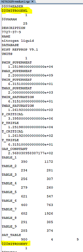
In Ansys Forte, usage of RGP table is limited to the gas phase (or "vapor") of a substance. The RGP table input file may contain more than one "material;" typically, this would be two phases (liquid and vapor) of a pure substance. Figure 3.13: RGP table input file: Nitrogen shows a screenshot of an RGP table input file for nitrogen. The RGP material names corresponding to liquid and vapor phases of nitrogen are
NITROGENLandNITROGENV, respectively. In the Equation of State settings, you need specify the RGP File Name by choosing the RGP table file from its location and select the RGP Material Name corresponding to the vapor phase (in this example, “NITROGENV”). The RGP material name for the liquid phase is irrelevant since the liquid data in the RGP file are not used by Forte.
Ansys Forte can simulate flow problems using either gas-phase or two-phase fluid, where "two-phase" refers to liquid and gas. By default, the working fluid is assumed to be in the gas phase. Here, the working fluid is referred to the continuous fluid filling the computational domain.
There are two types of simulations in which you can include liquid in the working fluid:
In the first type, while the working fluid as a continuum is in gas phase, you can set up Spray Model (see Spray Model) to simulate liquid droplets. Spray droplets are modeled as discrete particles, not as continuous fluid, and they interact with the gas phase as governed by several sub-models in the Spray Model settings. Even with the presence of sprays, we refer to this type of flow simulation as "gas-phase" since the continuous fluid is solely gas.
In the second type of simulation, the working fluid as a continuum can be liquid, or gas, or a mixture of both. It is referred to as Eulerian two-phase flow simulation. To use this approach, the liquid species must have been defined in the chemistry set. You can compile such a chemistry set using the Chemistry Set Pre-Processing Utility, and make sure that liquid species are defined in the surface kinetics input. Alternatively, you can use New Liquid & Vapor Pair (see Chemistry) to add the desired liquid species and let Ansys Forte automatically generate a chemistry set. Then, define a multiphase mixture (see Mixture Editor) as the working fluid, which can be used to specify the initial fluid compositions (see also Initialization Panel) and fluid compositions in certain boundary conditions (see also Inlet Panel). Once a multiphase mixture is used in an initialization and/or inlet, Forte automatically uses Eulerian two-phase flow simulation.
In an Eulerian two-phase flow simulation, a simple relation that considers compressibility effects is assumed for the liquid phase. The gas phase can be modeled by either the Ideal Gas or Real Gas model, depending on the settings for Equation of State as described in Equation of State. The settings for Equation of State are effective only for the gas phase in an Eulerian two-phase flow simulation.
The Global Liquid/Multiphase Settings on the Chemistry/Materials Editor panel is only meaningful in an Eulerian two-phase flow simulation. You have the option to select the Transport Model as Mixture Eulerian 2-Phase or Volume of Fluid. In the Mixture Eulerian 2-Phase model, liquid and gas are transported as a mixture without accurate tracking of the interface between the two phases. The Volume of Fluid model provides a more accurate interface-tracking capability.
When using the Mixture Eulerian 2-Phase model, you may select the Phase Change Option as No Phase Change or ZGB Finite-Rate Model. By definition, phase change is the process of local mass transfer between liquid and gas phases. When No Phase Change is selected, phase change is not considered, and the phase concentrations of the fluid are only affected by flow transport. When ZGB Finite-Rate Model is selected, local phase-change processes are simulated by the Zwart-Gerber-Belami model, which calculates local evaporation (or cavitation) and condensation effects by the theory of bubble growth and collapse. The four parameters of this model are the Bubble Radius (default: 1e-6 m), Nucleation Site Volume Fraction (default: 5e-4), Evaporation Coefficient (default: 50.0), and Condensation Coefficient (default: 0.01). The Bubble Radius is inversely proportional to both the rates of evaporation and condensation. The Nucleation Site Volume Fraction and Evaporation Coefficient affect evaporation only and are both proportional to its rate. The Condensation Coefficient affects condensation only and is proportional to its rate.
Note: Usage of ZGP Finite-Rate Model is allowed when the Equation of State is Ideal Gas or Real Gas. It is not allowed when the Equation of State uses RGP file.
In an Eulerian two-phase flow simulation, the gas phase is regarded as “free gas” by default, meaning that it is not dissolved in liquid and is modeled by gas’ thermodynamic relations. In certain applications, you might want to consider dissolved gas and the gas cavitation process, which accounts for mass transfer between the dissolved gas and free gas. Here, the distinction between dissolved and free gas is made only for non-condensable gas, defined as gas species that do not participate in phase change.
When using the Mixture Eulerian 2-Phase model, you may select the Gas Cavitation Option as No Gas Cavitation or Lifante Finite Rate Model. When No Gas Cavitation is chosen, the gas phase is assumed to be free gas. When Lifante Finite Rate Model is chosen, you may control the rate of mass transfer between the free gas and dissolved gas by four modeling parameters. Degassing Coefficient (default: 2.0) is proportional to the rate of mass transfer from the dissolved gas to free gas. Absorption Coefficient (default: 0.1) is proportional to the rate of mass transfer from the free gas to dissolved gas. Max Solubility Factor (default: 0.001) is a limiter on the absorption process such that if the dissolved gas’ mass fraction exceeds this value, absorption won’t happen. Henry Volatility Constant (default: 84028.0 Pa) is dependent on the fluid being considered and is used to compute an equilibrium pressure. Degassing happens when the local pressure is lower than the equilibrium pressure, and absorption happens when the local pressure is greater than the absorption pressure.
Note: The Eulerian two-phase flow simulation should not be used together with certain sub-models. In this type of simulation:
Activate Chemistry under Simulation Controls > Chemistry Solver should be Always Off.
Spray Model should be unchecked.
Spark Ignition should be unchecked.
Soot Model should be unchecked.
Radiation Model should be unchecked.
For inlet boundary conditions, the Temperature Option should not be Assume Isentropic. The Inflow Mixture Density Option should not be either Specify Total Density, Constant, or Specify Total Density, Time Varying when the Inlet option is one of these values:
Velocity
Velocity, Time Varying
Mass Flow Rate
Mass Flow Rate, Time Varying
When using the Mixture Eulerian 2-Phase model, an additional Phase Change Option, Phase Equilibrium is also available as a Beta feature. This option models local phase-change processes by a thermal equilibrium approach. Its use does not require you to specify any modeling parameter.
Note: Usage of Phase Equilibrium Model is allowed when the Equation of State is Ideal Gas. It is not allowed when the Equation of State is Real Gas or uses RGP file.
Ansys Forte can model flame propagation processes in a gas-phase and reacting flow simulation. After a chemistry set is imported, you will see Flame Speed Model under Chemkin Chemistry Set in the Workflow tree. Forte has several options for specifying the flame speed that can be accessed on the Flame Speed Model panel. The laminar flame speed can be calculated either by using formulations of the power law, or by using pre-calculated flame-speed tables. Turbulent flame speed is determined from a correlation, which takes the calculated laminar flame speed as well as several turbulence parameters as inputs. These concepts are described in Turbulent Flame Propagation Model of the Ansys Forte Theory Manual.
The recommended option for specifying flame speed is the Table Library option. These contain precalculated laminar flame-speed tables for 44 surrogate fuels. The fuels covered in the Table Library option represent several classes: families of n-alkanes, iso-alkanes, cyclo-alkanes, alkenes, cyclo-alkene, iso-alkene, aromatics, ethers, cyclo-ethers, alcohols and methyl esters. The fuels are listed in Table 1: Fuels for which prebuilt laminar flame speeds are available as part of the Table Library option. Using pure-fuel flame speeds and local fuel composition in the CFD simulation, multi-component-fuel flame speeds are calculated on-the-fly using non-linear blending of the single-component values. This Table Library option provides (a) simplicity in the input required for the CFD simulation (only fuel composition is required); (b) a high degree of accuracy afforded by the Ansys Chemkin-generated flame-speed library for an extensive range of fuel components; and (c) the automation of the blending without compute performance penalty.
The second option for specifying laminar flame speed is the flame-speed look-up table. The look-up table is a file that contains a series of flame table data points used to interpolate to the correct flame speed and can be edited with the Profile Editor. For details on working with the flame-speed table, see Flame-Speed Table Editor. Lookup tables for five surrogate fuels are provided with Ansys Forte, and these can be used as templates when you want to build your own laminar flame-speed tables.
The third option is the power-law option, for which further options are provided when selecting the Flame Model and its Speed at Reference State, Temperature and Pressure Dependency, and Diluent Effect.
The model inputs for the Turbulent Flame Speed correlation are also listed in this Flame Model panel. Their meanings are explained in the tool tips. More details are described in Ansys Forte Theory Manual.
User Defined Functions (UDF) for laminar and turbulent flames (see also User Defined Functions (UDF))
Laminar and turbulent flame speed correlations can also be defined through User Defined Functions (UDFs). This option is provided as the last item on the and drop-down lists. For detailed information about how to use Ansys Forte UDFs, see the README.txt file in the user_defined_functions directory in your Ansys Forte installation. Template UDF source code for the flame speed models is provided in the combustion subdirectory. The interface parameters for the UDFs are described in the template code. For the language used in writing the UDFs, both Fortran and C/C++ are supported. The UDFs in the combustion subdirectory will be compiled into a dynamic link library, libForteUDF_combustion.dll, on Windows, or a shared object, libForteUDF_combustion.so, on Linux systems.
Note: Do not change the names for the .dll or .so files because this naming convention is used by the Forte executable.
The input and output parameters for the flame-speed UDFs are listed below.
1. UDF_Combustion_LaminarFlameSpeed
Inputs
pressure – pressure of the unburned gas mixture, unit is
[dynes/cm2]
temperature – temperature of the unburned gas mixture, unit is
[K]
nSpecies – number of gas-phase species in the chemistry
mechanism
nElement – number of elements in the chemistry mechanism
kO2 – species index of O2 (1-based, that
is, the index of the first species is 1. The value is 0 if this species does not exist in the
mechanism.)
kCO2 - species index of CO2 (1-based)
kH2O – species index of H2O
(1-based)
kN2 – species index of N2 (1-based)
keleH - element index of H (1-based)
keleC - element index of C (1-based)
keleO - element index of O (1-based)
keleN - element index of N (1-based)
eleNum - elemental composition of gas species. The dimension is (nElement,
nSpecies) in Fortran and [nSpecies] [nElement] in C/C++. It returns the number of element
i in species j.
molecularWeight - molecular weights of all gas species, unit is [g/mol]
massFraction – species mass fractions of the unburned gas mixture
Outputs
laminarFlameSpeed -- laminar flame speed, unit is [cm/s]
iError -- 0 if there is no error, other value if there is error
2. UDF_Combustion_TurbulentFlameSpeed
Inputs
pressure - pressure of the unburned mixture, unit is
[dynes/cm2]
unburnedTemperature - temperature of the unburned mixture, unit is
[K]
equilTemperature - equilibrium temperature of the flame following a constant
pressure, constant enthalpy process, unit is [K]
laminarFlameSpeed - laminar flame speed, unit is [cm/s]
laminarFlameThickness - laminar flame thickness, unit is [cm]
turbulentKineticEnergy - turbulent kinetic energy, unit is
[cm2/s2]
dissipationRate - dissipation rate of turbulent kinetic energy, unit is
[cm2/s3]
integralLengthScale - turbulence integral length scale, unit is [cm]
timeElapse - time elapsed since spark timing, unit is [s]
Outputs:
turbulentFlameSpeed - turbulent flame speed, unit is [cm/s]
iError - 0 if there is no error, other value if there is error
integralLengthScale - turbulence integral length scale,
unit is [cm]
timeElapse - time elapsed since spark timing, unit is
[s]
Chemistry in Flame Front Region: When the flame front is tracked with the G-equation, the chemistry in the flame front region determines the heat release and species evolution, including emissions. Details on chemistry in the flame front region are described in the G-equation Model in G-equation Model in the Ansys Forte Theory Manual. Two options are provided for describing the chemistry in the flame-front region: Equilibrium and Stirred-reactor model (patent pending) [29]. When the Equilibrium option is chosen, no further inputs need to be specified. When the Stirred-reactor model option is chosen, residence time can either be dynamically calculated or user-specified.
Use Legacy G-Convection Formulation: This check box provides backwards compatibility to a previous (prior to the R18.1 release) model for determining the mean flow convection term in the G transport equation. The default G convection formulation is recommended for flame propagation cases involving especially large mean flow velocities; for example, under high-swirl engine operating conditions. This affects how the flame surface (represented by the G=0 iso-surface) is transported, considering both the flame propagation speed and the mean flow velocity.
If the legacy option is selected, the mean flow velocity used in the formulation will be the value on the flame-front surface and the expansion effect is accounted for in the flame-speed term.
If the legacy option is not selected, that is, the default formation is used, the mean flow velocity will be the value on the unburned side of the flame front and the expansion effect is accounted for by the mean flow velocity term. Since the mean flow convection effect is ignored during the ignition kernel stage when using the legacy formulation, the default formulation is the preferred option. Using the default formulation requires a higher value for the turbulent-flame-speed ratio (b1) value in the turbulent-flame-speed correlation, typically 2x the value used with the legacy formulation.
Unburned Calculation Method: Three different options are provided for picking unburned conditions in the flame propagation models. The Find Nearest Unburned Cell without Volume Search option takes the unburned condition picked in the immediate neighborhood of the flame front. The Volume Search with Fixed Radius option picks the unburned condition a fixed distance away from the flame front, which prevents the unburned condition from being influenced by the hot burned gas inadvertently. The Volume Search with Variable Radius option also uses a volume search, similar to the second option. But instead of using a fixed search radius, it uses a variable search radius that scales with the local cell size. The latter two options make the laminar flame speed calculation less sensitive to mesh resolution. To obtain equivalent burn rate results, the latter two options require a larger flame development coefficient (up to 2x) compared to the option without volume search, especially for slow-burning cases.
Use Legacy Method For Flame Front and High-Temperature Front Synchronization: In release 2020 R1, a new default method is used to overcome a modeling difficulty in the G-equation flame propagation model that may occur under certain operating conditions. When the unburned temperature is high and flame speed is low, strong thermal diffusion can cause the high-temperature front to propagate faster than the flame front surface marked by the G=0 iso-surface and cause these two surfaces to become out of sync. The new default method is devised to keep these two surfaces in sync should they show a tendency to separate. It is recommended that the default option be used for all new Forte projects. The legacy option, enabled using this check box, is provided only to maintain backward compatibility. Clear this check box to use the improved treatment.
Disable Flame Propagation Model: These options allow the flame propagation model to be turned off by a user specification to avoid solving the flame propagation model equations unnecessarily during certain time or crank angle range of a calculation. These options are especially useful in engine simulations. If When an Engine Cylinder is Not a Closed System is selected, the flame propagation model will be disabled as soon as any port or valve is open in a cylinder region. This is the default and recommended option. If After User-Specified Crank Angle or Time is selected, the flame propagation model will be disabled after the specified timing. The model will be reactivated at spark timing of the next engine cycle in engine cases. If Never is selected, the flame propagation model will keep being solved until the flame quenches by itself.