


This section reviews the best practice of simulating rotary-lobe compressors in Ansys Forte.
Related Tutorials:
While the tutorials provide specific examples of the rotary-lobe compressors and focus on their settings, the present section emphasizes the general best practice and tips. We will use the compressor in Rotary Lobe Compressor Simulation in the Ansys Forte Tutorials (which is a Roots-type blower) to illustrate the concept. The same concept also applies to:
Screw compressors
Gear Compressors
Other compressor types involving two engaging rotors
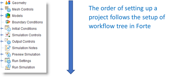
As in any simulation using Ansys Forte, it is recommended that you follow the order of the Simulation Workflow tree to set up a compressor simulation:
Therefore, the content of this section is arranged as follows:
Surface Geometry Import
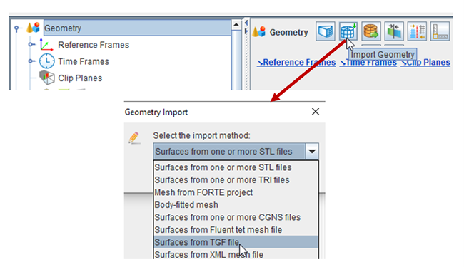
Suppose that you have prepared the surface geometry in Ansys Discovery or SpaceClaim in the .tgf format. To import the geometry into Forte, go to Geometry > Import Geometry, as illustrated in Figure 5.17: Import Geometry in Forte Simulate User Interface. Select the import method as Surfaces from TGF file.
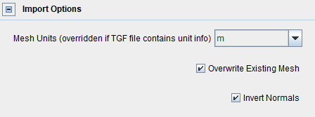
In Import Options, pay attention to the Mesh Units. Make sure that the unit is consistent with the one used when the surface geometry is created. Select Invert Normals. Why the normals need to be inverted will be explained in the sub-section Surface Normal Requirements in Compressor Simulations.
Visualize Surface Mesh Lines
After the surface mesh is imported, you may select all named surfaces in the
Geometry tree (use the shift or
ctrl keys to multi-select). On the right-click menu, toggle on
"Mesh" to display the surface mesh lines on the surfaces. Use
the "light bulb" icon ![]() in front of each surface or toggle Visible
to change its visibility.
in front of each surface or toggle Visible
to change its visibility.
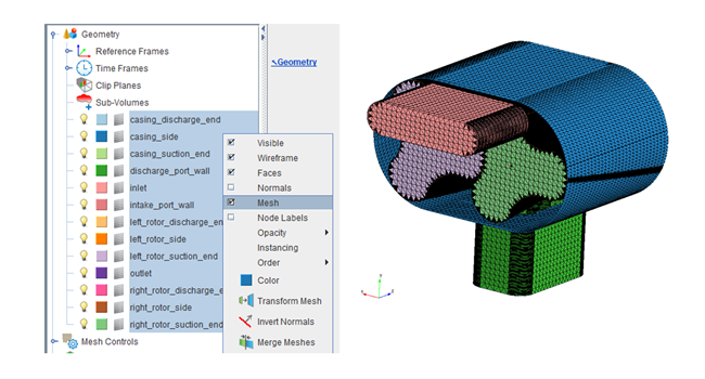
This is an optional but very helpful step to examine the surface mesh resolution and to see whether it is too fine or too coarse. Note that when the surface mesh is written as .tgf file, there is no chance to see the mesh lines until the geometry is imported and visualized in the Forte Simulate User Interface (UI). For general guidance on the proper surface mesh resolution, refer to Surface Mesh Generation.
Surface Normal Requirements in Compressor Simulations
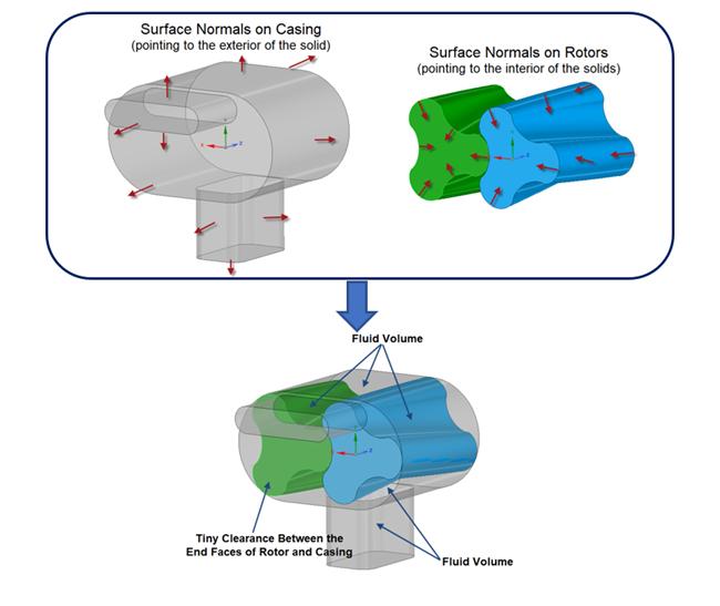
When the compressor's rotors, casing and ports assembly are created in Ansys SpaceClaim, they are created as "solid" volumes and the surface normals point to the interior of the solids. The .tgf file exported from SpaceClaim follows the same convention on the normal directions.
When the .tgf file is imported into Forte, as mentioned above, turning on the Invert Normals option is recommended. Having done so, all the surface normals now point to the exterior of the "solid" volumes.
To do a CFD simulation in Forte, surface normals are always required to point to the EXTERIOR of the fluid volume. This means that,
For the casing and ports assembly, normals should point to the exterior of the "solid" - no further action is needed.
For the rotors, normals should point to the interior of the "solid" - the normals should be inverted (see below).
This requirement is illustrated in Figure 5.20: Surface Normals on the Casing, Ports, and Rotors Surfaces that Meet the Requirement of Forte.
Caution: Incorrect (flipped) surface normal is one of the most common setup errors!
Figure 5.20: Surface Normals on the Casing, Ports, and Rotors Surfaces that Meet the Requirement of Forte
Normals represented by small red arrows can be displayed by right-clicking the surfaces and toggling Normals. To invert the rotor surfaces, choose Invert Normals for these surfaces. (See Figure 5.21: Invert Normals on the Rotor Surfaces.)
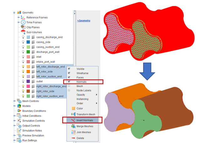
Note: If you import a modified geometry to replace the old one, remember to repeat the Invert Normals operation for the rotors because the normals won't be inverted automatically in the geometry replacement process.
Create Small Gaps Between Surfaces
In compressors, gaps exist between the rotors as well as between the casing and the rotor. As mentioned in Small Gap Handling, gaps are critical to the simulation of compressors since they affect the prediction of fluid delivery and flow leakage.
If the surface geometry in your Forte project already contains gaps that are true to the actual compressor, you can skip this step.
However, if there are no gaps between rotor and casing or between the two rotors in the imported geometry, you can use the method described here to create the gaps. In this example, a gap of around 70 micron will be created by shrinking the sizes of the rotors along their radial directions.
Note: When you shrink the sizes of the rotors, you are creating (or enlarging) the gaps between them and between the rotor and the casing.
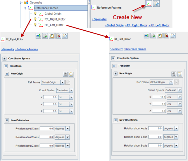
First, to facilitate the geometry transformation, create two Reference Frames to anchor the two rotors' axes. This is illustrated in Figure 5.22: Creating Two Reference Frames to Anchor the Two Rotors' Axes. In this example, the two reference frames created are named "RF_Right_Rotor" and "RF_Left_Rotor". The Orientation of the reference frame must be aligned with the rotor's axial direction. The Origin of the reference frame must be on the rotor's axis. Typically, the two reference frames' origins have some distance apart (in this example, 12 cm), but have the same orientations, because the two rotors are co-axial.
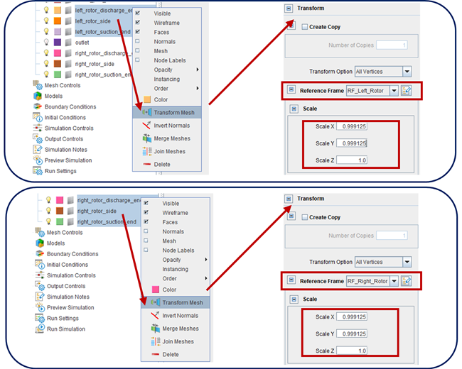
Next, the sizes of the two rotors will be shrunk. This is done for each rotor separately, as illustrated in Figure 5.23: Shrinking the Sizes of the Two Rotors. Select all the surfaces that constitute one rotor and use Transform Mesh. On its panel, set the Reference Frame to the one anchoring on this rotor, and set the Scale factors in each direction (-X, -Y, and -Z). The rotor's axis is in the -Z direction, so, the shrinking is applied only in the -X and -Y directions, with respect to the rotor's own reference frame.
The scale factor is calculated as:

In which 0.007 cm is the target gap size between the rotor edge and casing, and 8.0 cm is the original rotor radius.
Note: The method of enlarging the gaps by shrinking the rotors' sizes are also applicable when dealing with surface mesh intersection issues. See Resolve Assertion Failure or Surface Intersection in a Screw Compressor.
Material Point
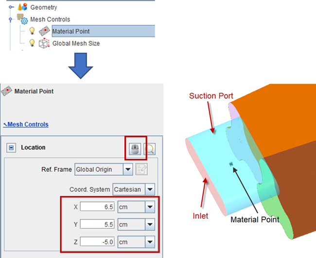
As in any Forte simulation, the Material Point must be always inside the fluid domain. Its location does not have to be precise, but it must be at least one unit cell length away from all boundaries.
In a compressor simulation, certain boundaries, such as the rotors, can move. This must be considered when placing the material point. Here, a method to put the material point in the compressor's suction port is shown, which is static during the simulation. To do so, a point on the "inlet" surface is hand-pick, and then the Z-coordinate is increased to move it into the suction port. This is illustrated in Figure 5.24: Placing the Material Point in the Compressor's Suction Port.
To hand-pick a point on geometry, first click the mouse icon ![]() on the Material Point panel, and then hold
'Ctrl' and click the target location on the geometry. In this example, target the
mouse click at the center of the "inlet" surface.
on the Material Point panel, and then hold
'Ctrl' and click the target location on the geometry. In this example, target the
mouse click at the center of the "inlet" surface.
Then, move the point location into the suction port by increasing the z-coordinate.
Tip: The Material Point can be visualized by toggling on the
light bulb icon ![]() next to Material Point on the workflow
tree.
next to Material Point on the workflow
tree.
Global Mesh Size
Global Mesh Size depends on your compressor size and the size of fluid domain to simulate. It is generally recommended that the total cell count in a compressor simulation should be smaller than 1 million. Typical global mesh size range is 1 to 4 mm.
Surface Refinement Controls for Inlet and Outlet
It is recommended to add mesh refinement controls near the open boundaries of your
simulation domain: the inlet and outlet of the compressor. Click Mesh
Controls in the workflow tree and click the New Surface Depth
Refinement icon ![]() . The panel is shown as in Figure 5.25: Adding a Surface Depth Refinement Control for Inlet and Outlet.
. The panel is shown as in Figure 5.25: Adding a Surface Depth Refinement Control for Inlet and Outlet.
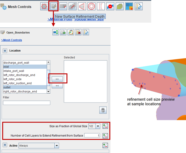
Here, multi-select inlet and outlet so that the refinement applies to the meshes near both boundaries. Set Size as Fraction of Global Size to 1/2, so that the refined mesh size is half of the global mesh size. Set Number of Cell Layers to Extend Refinement from Surface to 1. Set the Active duration to Always.
After this mesh control is set up, its light bulb icon ![]() in the workflow tree can be used to preview the corresponding
refined cell size at sampled locations on the affected boundaries. This is shown on
the inlet boundary in Figure 5.25: Adding a Surface Depth Refinement Control for Inlet and Outlet.
in the workflow tree can be used to preview the corresponding
refined cell size at sampled locations on the affected boundaries. This is shown on
the inlet boundary in Figure 5.25: Adding a Surface Depth Refinement Control for Inlet and Outlet.
Surface Refinement Controls for Wall Boundaries
In a compressor simulation, there are so-called "End Wall" and "Side Wall" boundaries. See Figure 5.26: End Wall and Side Wall Boundaries in a Compressor Simulation for some denotations of both.
End Walls refers to the wall boundaries at the two axial ends of the rotors. This is where the rotor's axial end meets the casing wall and forms a very small gap. In this figure, the end walls of the left rotor, the right rotor, and the casing are denoted. Note that only the end walls close to the inlet are denoted. There are end walls of the rotors and casing at the other end of the rotor axis.
Side Walls refer to all the other wall boundaries that are not regarded as end walls. These include the side wall of the casing (denoted in the figure), the side walls of the rotor surfaces, and the walls of the suction and discharge ports.
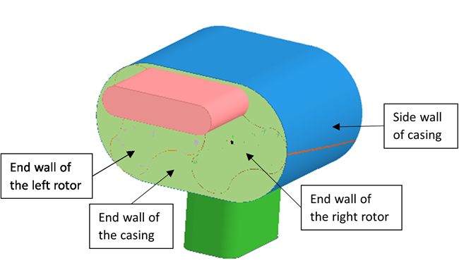
It is recommended to add Surface Depth Refinement for all the wall boundaries. The settings are similar to the ones used for the open boundaries. The Size as Fraction of Global Size is recommended to be 1/2 for all the side walls and 1/4 for all the end walls.
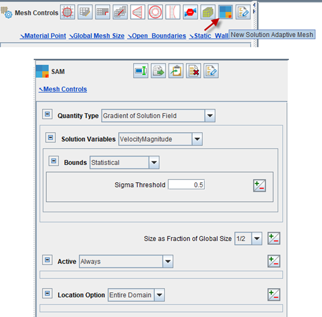
Solution-Adaptive Mesh Refinement
In a compressor simulation, it is recommended to add a Solution Adaptive Mesh (SAM) control based on the flow velocity gradient. As illustrated in Figure 5.27: Solution-Adaptive Mesh Refinement based on Flow Velocity, set the Quantity Type as Gradient of Solution Field, and set the Solution Variables as VelocityMagnitude. Set the Bounds as Statistical and the Sigma Threshold to 0.5. The Size as Fraction of Global Size is set to 1/2.
Gap Feature Controls
In a rotary-lobe compressor, there are small gaps formed between the two rotors and between each rotor and the casing wall. As explained in Small Gap Handling, it is critical to simulate the flows through these gaps. Gap Feature mesh controls and mesh refinement are required for both the rotor-rotor and the rotor-casing gaps to make sure these small gap regions are filled with fluid cells.
Therefore, for a rotary-lobe compressor, at least three Gap Feature mesh controls are needed, as illustrated in Figure 5.28: Three Gap Feature Controls Used for Rotor-Rotor and Rotor-Casing Gaps. Each gap feature control requires exactly one pair of surfaces (two surfaces). There is one control for the gap between the left rotor (left_rotor_side) and the casing (casing_side) surfaces, one control for the gap between the right rotor (right_rotor_side) and the casing surfaces, and one control for the gap between the two rotors.
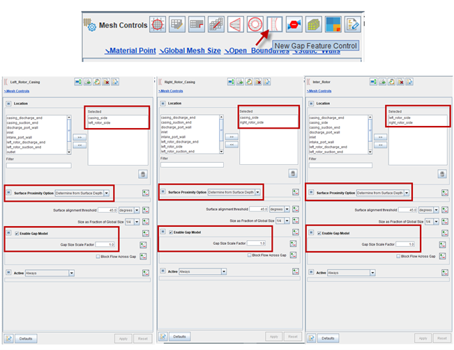
Surface Proximity is used as an important criterion for identifying gap zones. It is strongly recommended that you choose the default option Determine from Surface Depth.
Note: If you choose to set Surface Proximity manually (which is not recommended), refer to the guidance in Set Surface Proximity Manually in Gap Feature Meshing Control.
The smallest geometric spacing between these gaps is usually much smaller than the fluid cell size in the gap region. It is necessary to Enable Gap Model and let the gap model compensate for the under-resolution of the gap size.
The Gap Size Scale Factor in the gap model can be used to adjust the gap size measured in the geometry. The best practice is to keep the gap size scale factor as 1.0 (the default). If the gaps have been artificially modified in the surface geometry (for example, to avoid surface mesh intersection as explained in Resolve Assertion Failure or Surface Intersection in a Screw Compressor), this factor can be used to scale the sizes back to the true size.
This scale factor can also be used to study the gap size effect on the compressor's performance. Smaller gap size increases flow resistance across the gap and reduces leakage.
Import Chemistry Set
The first thing to set up the models is to import a "chemistry" set. This allows you to define compositions and properties of the working fluid and chemical reactions (if any). For compressor simulations, there is no chemical reaction involved, but you still need a chemistry set to define the working fluid.
If the working fluid of the compressor is air, from the Chemistry/Materials panel, select New Import Chemistry, and import Air_NoReactions_2sp.cks. This chemistry set file can be found in your Forte installation's directory:
/ANSYS Inc/v242/reaction/forte.***/data
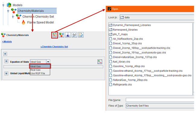
For air compressors, choose Ideal Gas as the Equation of State option.
For refrigerant compressors, refer to Refrigerant Properties about the appropriate chemistry set and Equation of State option.
Define the Fluid Mixture
You may now set up a fluid mixture for the working fluid. This will be helpful in defining the fluid composition in initial conditions and inlet boundary conditions.
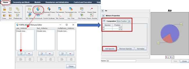
To set air as the working fluid, use the Mixture Editor located under Home > Libraries > Mixtures, as shown in Figure 5.30: Set up a Mixture for Air as the Working Fluid. In this case, you want to create a gas mixture. On the mixture editor, use Add Species to add o2 and n2 to the mixture. Set Mole Fraction of o2 to 0.21 and n2 to 0.79, respectively. Give this mixture a name (Air) and save it for later use.
Note: The Mixture Editor is introduced in more detail in Mixture Editor in the Ansys Forte User's Guide.
Physics Models
In compressor simulations, it is recommend to use the RANS RNG k-epsilon model for turbulence (Models > Transport > Turbulence) with all its default parameters.
There is no need to set up other models for this type of application.
Inlet
In a rotary-lobe compressor, an inlet boundary is located at the suction port.
Go to the Boundary Conditions node from the workflow tree, and choose New Inlet to add an inlet boundary condition. Use the mixture Air as the inlet fluid's Composition. Select the inlet surface from the geometry as Location.
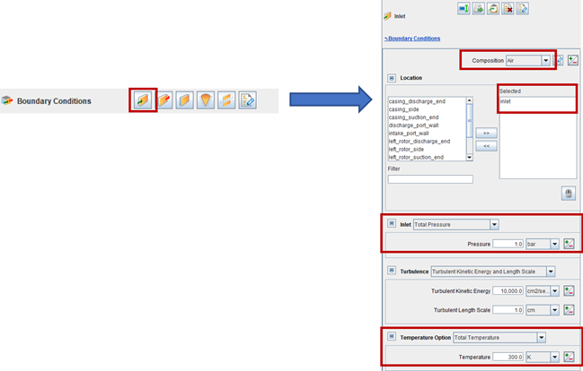
For the Inlet option, it is recommended to set Total Pressure or Static Pressure. Total Pressure is preferred, because it helps suppress inhomogeneity of the flow rate and flow re-circulation on the boundary. For the Temperature Option, set the Total Temperature. Keep the default Turbulence settings.
Caution: Pay attention to the units of the boundary parameters. Incorrect units are frequently encountered setup errors.
Outlet
In a rotary-lobe compressor, an outlet boundary is located at the discharge port. To define its boundary condition, it is recommended to use the New Inlet rather than the New Outlet option. The main reason is that the Inlet option allows the composition, pressure, and temperature of any reverse flow to be explicitly specified. Reverse flow, or backflow, is quite common during a compressor simulation. As discussed in Prevent Backflow, it is hard to eliminate backflow completely in such a simulation.
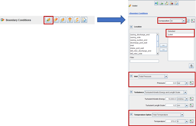
Use the mixture Air as the backflow's Composition. Select the outlet surface from the geometry as Location. For the Inlet option, it is recommended to set Total Pressure or Static Pressure. Total Pressure is preferred because it helps suppress inhomogeneity of the flow rate on the boundary. For the Temperature Option, set the Total Temperature. Keep the default Turbulence settings.
Note: In a compressor simulation, pressure and temperature at the outlet boundary are typically larger than those at the inlet boundary.
Note: You may also use the Outlet boundary condition for the outlet. When specifying pressure at the open boundary, the usage of Inlet and Outlet types does not make much difference, except that with the Inlet type you could specify temperature in the ghost cell outside the boundary while the Outlet type does not allow it. Using the Outlet type, the temperature in the ghost cell is set the same as that in the interior cell. When backflow happens, the treatment using the Inlet type makes more sense. This is why using the Inlet type for outlet boundaries is recommended for such situations.
Static Walls
In a rotary-lobe compressor, static wall boundary conditions are typically set for the following surfaces:
Suction Port
Discharge Port
Casing
Go to the Boundary Conditions node from the workflow tree, and choose New Wall to add an inlet boundary condition. For static walls, do not turn on the Wall Motion. You may activate Heat Transfer and set Wall Temperature on these walls.
Moving Walls
Now the moving wall boundary conditions for the two rotors in the compressor must be set. These are illustrated in Figure 5.33: Moving Wall Boundary Condition for the Left Rotor and Figure 5.34: Moving Wall Boundary Condition for the Right Rotor.
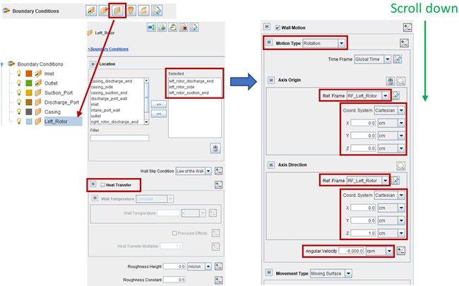
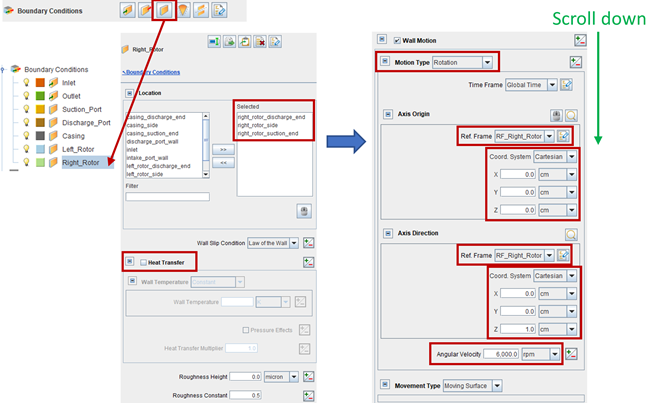
Recall that each rotor might include a side wall and two end walls, and they all need to be selected in the boundary condition definition. You may use adiabatic boundary conditions by deactivating Heat Transfer on the rotors. The rotors are typically completely enclosed in the casing and they are not cooled or heated, so under steady operation, they should reach an equilibrium state (same temperature on average) with the working fluid surrounding them.
Turn on Wall Motion and choose the Motion Type as Rotation. Here, you need to define the Axis Origin and Axis Direction for the rotation. In this example, two Reference Frames have been created, centered at the axes of the two rotors, respectively. Setting up the axis origin and direction with respect to the reference frame is easier. More information about the reference frame can be found in Reference Frames in the Ansys Forte User's Guide.
Specify the Angular Velocity for the rotation. The sign of the angular velocity follows the right-hand rule regarding the rotation axis.
Set the Movement Type as Moving Surface.
A rotary-lobe compressor simulation typically involves only one region in terms of initialization. Go to Initial Conditions in the workflow tree and click Default Initialization. Set the Composition of the working fluid. In this example, the mixture Air defined earlier can be used. Then, set the initial Temperature and Pressure. You may leave the Turbulence quantities as the default and set the initial Velocity to zero.
Simulation Duration
To set the simulation duration, go to Simulation Controls in the workflow tree. On its main panel, choose Time Based as the Simulation End Time Option, and set the Max. Simulation Time.
Note: A compressor simulation typically goes through the initial transient process and stabilizes after 2 to 3 revolutions of rotors.
Tip: The time for each revolution is calculated as 60/RPM [second].
Time Step Control
It is necessary to determine the maximum time step size. This is specified by Simulation Controls > Time Step > Max. Time Step Option. For compressor simulations, it is recommended that you set the maximum step size to correspond to roughly 0.1 degrees of rotation.
This is calculated as 1/(RPM*60) [second]. For example, if the RPM of rotor rotation is 6000, then the max time step size is calculated as 2.78E-6 s.
Ansys Forte uses an automatic time stepping technique. The time step is automatically adjusted during the simulation to account for stability and efficiency. The adjustment can be influenced by changing the Advanced Time Step Control Options on the Time Step panel. It is typically acceptable to increase (for example, double) the Fluid Acceleration Factor and Rate of Strain Factor to allow larger time step size to be reached. However, it is recommended NOT to increase the Convection Factor because it may result in solution instability.
Chemistry Solver
This simulation does not involve chemical reactions. On the Simulation Controls > Chemistry Solver panel, change Activate Chemistry to Always Off.
Spatially Resolved Outputs
Spatially resolved outputs allow you to examine the flow solutions in detail. Select Time as Output Timing Control. The Interval Based Output Control sets a fixed output frequency. For example, a 0.0005 second interval provides 20 results for one revolution at 6000 RPM. The User Defined Output Control allows you to create a customized time value list to save solutions for a specific time range to get higher output resolution in that range.
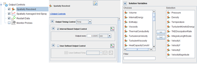
In the Solution Variables list, you may include or exclude any variables in the output files. It is recommended to only keep the solution variables of interest to minimize the output file size. The key output variables in a rotary-lobe compressor simulation are shown on the selection list in Figure 5.35: Spatially Resolved Panel in Output Controls. Considering the typical mesh size in such simulations, the size of each solution file is typically on the order of 100 - 500 MB.
Spatially Averaged Outputs
The spatially averaged output settings are on Output Controls > Spatially Averaged and Sprays. Select Time as the control option. The size of spatially averaged output files are relatively small. It is acceptable to save results at high frequency, but the interval should be larger than the time step. A standard set of spatially averaged output variables will be reported in various .csv output files. You may select species n2 and o2 in the Spatially Averaged Species list to monitor their total mass in the domain.
Pocket Tracking is a useful output control that can be enabled on the same panel. Refer to Pocket Tracking in the Ansys Forte User's Guide for its usage.
Restart Controls
Output Controls > Restart Data manages the restart data writing.
Make sure that Write Restart File at Last Simulation Step is checked. A restart file saved at the end of a run is useful for doing parameter studies by running additional revolutions afterwards. In this case, using the restart file helps save CPU time by bypassing the initial transient process.
Interval Based Restart helps provide a recovery point if a long-running case crashes for any reason. For example, you may set an interval-based restart to be written for every 500 timesteps. As soon as a new interval-based restart is created, the previous one will be deleted such that only the latest one is kept. This is a measure designed to save disk space.
You can also specify specific time values for saving restart using User Defined Restart Points. Select Time as the Time Option if you decide to turn on this option.
Monitor Probes
In compressor simulations, monitor probes are helpful for monitoring pressure and temperature evolution at selected locations. Turn on Monitor Probes under Output Controls. For Inquiry Frequency, use Time as the option and set Output every to an interval similar to that used in the spatially averaged output.
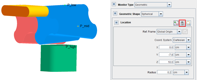
In Figure 5.36: Use Spherical Monitor Probes to Inquire Local Solutions, three monitor points are set
up. P_low is located on the suction side,
P_mid is in the compression chamber, while
P_high is close to the discharge port. Select
Geometric as the Monitor Type, and select
Spherical as the Geometric Shape. Specify
the Location of the monitor probe. If you are not sure about
its exact coordinates, click the mouse icon ![]() , hold 'Ctrl', and click a target location on the surface
geometry to get approximated coordinates, and then fine-tune the coordinates. To
monitor local solutions, the Radius of the monitor probe can be
equal to or slightly larger than the Global Mesh Size.
, hold 'Ctrl', and click a target location on the surface
geometry to get approximated coordinates, and then fine-tune the coordinates. To
monitor local solutions, the Radius of the monitor probe can be
equal to or slightly larger than the Global Mesh Size.
You may select any supported Solution Variables to be monitored, but pressure and temperature are typically selected.
Monitor probes of this type are static and they do not move with the rotor surfaces. Make sure that there are always fluid cells within the probe radius to get meaningful solutions from the local flow field. Therefore, in this example, their locations are chosen to be next to the casing surface so that they can inquire the fluid cells in the gaps when the rotors sweep by.
There are many other types of monitor probes in Ansys Forte, one of which is based on boundary conditions. You can monitor parameters averaged over a boundary condition by choosing Boundary Condition as the Monitor Type. For example, such a monitor probe can be used to monitor the temperature and pressure averaged at the Outlet boundary.
Mesh Preview Using Ensight
After setting up the simulation following the aforementioned steps, you are now ready to validate the project's settings. Since the compressor simulation always involves moving boundaries, it is recommended to do a Mesh Preview before running the simulation. Mesh Preview allows you to check the validity of the boundary motion and make sure that the surface meshes do not intersect each other during the transient simulation. The procedure of mesh preview is illustrated in Figure 5.37: Mesh Preview and View the Results in EnSight.
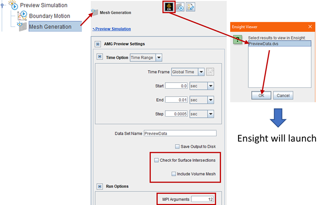
Use the Time Option to specify the time range and intervals to generate the preview mesh. It is recommended placing sufficient (but not too many) instances to cover at least one revolution of the rotors. In this example, RPM is 6000, and each revolution takes 0.01 s. Using a Step size of 0.0005 s, 20 instances will be generated.
To preview the boundary motion only, use the default settings.
If you like to check for potential surface intersections, turn on Check for Surface Intersections. This option would take slightly longer CPU time, so it is better to run in parallel mode (by increasing the value of MPI Arguments, which is the number of cores).
If you like to check the volume mesh, turn on Include Volume Mesh. Volume mesh generation takes even longer CPU time. It can be used to check the mesh at a particular time moment (like a "snapshot"), if needed.
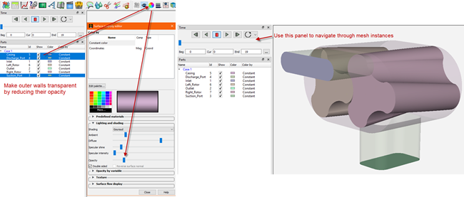
Visualize Boundary Motion
Clicking the Launch Ensight button ![]() on the Mesh Generation panel opens the
mesh results in Ansys EnSight. To visualize the boundary motion, multi-select the
surfaces corresponding to the casing, the suction and discharge ports in the
Parts list, open the Color/Transparency
panel, and reduce their opacity to make them transparent. This allows you to see the
rotors more clearly. Use the Time navigation panel to navigate
through mesh instances and observe the rotors' motion.
on the Mesh Generation panel opens the
mesh results in Ansys EnSight. To visualize the boundary motion, multi-select the
surfaces corresponding to the casing, the suction and discharge ports in the
Parts list, open the Color/Transparency
panel, and reduce their opacity to make them transparent. This allows you to see the
rotors more clearly. Use the Time navigation panel to navigate
through mesh instances and observe the rotors' motion.
Check for Surface Intersections
Surface intersection is what should be avoided in a Forte simulation. When surface intersection occurs during the simulation, it could cause the simulation to crash (see Error Caused by Surface Intersection (Assertion Failure)). In a compressor simulation, due to the small gaps between the moving rotors and between the rotors and the casing, surface intersection is more likely to occur if the geometry and/or boundary motion are not set up correctly.
If you have turned on Check for Surface Intersections on the Mesh Generation panel, you will see a part called intersections in the Parts list. The intersection points, if any, are marked as crosses (refer to Figure 3.6: Surface intersections viewed using cut planes). You might need to hide all other parts and only keep intersections to see them clearly. Use the Time navigation panel to navigate through mesh instances and observe the potential intersections.
If you see some intersections, you can examine them more closely.
First, visually identify which surfaces are causing the intersections. In a compressor simulation, they are most likely caused by the two rotor surfaces and the casing.
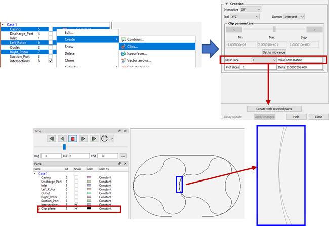
Then, create a clip plane and let it cut through the surfaces causing the intersections. In the example given in Figure 5.39: Using a Clip Plane to Examine Surface Intersections Closely, with "Casing", "Left_Rotor", and "Right_Rotor" multi-selected, right-click to create a clip plane (Clips…). Since the rotors' axial direction is Z, we choose Z for Mesh slice, set its Value to the locations of interest, and click Create with selected parts. A new part called Clip_plane is created.
Color Clip_plane by black to make it easily visible. Set the
view orientation to Z+ using the ![]() icon at the bottom of the graphic window. Zoom in to see
details of potential intersections in the gap zone.
icon at the bottom of the graphic window. Zoom in to see
details of potential intersections in the gap zone.
The curves of different surfaces should not intersect into one another in any way. If you see them intersect, that indicates problem, and it should be fixed. Figure 3.6: Surface intersections viewed using cut planes shows an example of what intersected surfaces look like.
You may change the Z location of the Clip_plane to check intersections at different locations along the axial direction. Do the same check for all mesh instances using the Time navigation bar.
Fix Surface Intersections
If intersections are identified, below are common causes:
The positions of the rotors in the geometry are incorrect.
The specified locations of the rotation axes are incorrect.
The facets on the side surfaces of casing and rotors are too coarse. This is related to the best practice about surface mesh generation. As mentioned in Surface Mesh Generation, when exporting the .tgf file in SpaceClaim, typically, control angle = 4° is adequate. You may reduce the control angle to increase the resolution of the facets.
Note: Generally, it is recommended to fix all the surface intersections observed in Mesh Preview. Sometimes, the intersections are benign, but it is very difficult to say when. Depending on the dynamic mesh refinement and how it might change during the simulation through motion or solution adaption, the intersections could become a problem at any time, so it is somewhat of a gamble to run with them. If you encounter meshing-related error during the simulation, as discussed in Error Caused by Surface Intersection (Assertion Failure), it is always good practice to re-visit the Mesh Preview procedure discussed here, check, and fix the intersections.