


This tutorial describes how to use Ansys Forte CFD to simulate the flow processes in a positive-displacement twin-screw compressor with oil injection. The tutorial covers the usage of a Volume-of-Fluid two-phase model in Forte to simulate the multiphase flows in this type of application.
This document will go through all the simulation setup steps, with emphasis on the following aspects that are unique or important to the oil-injected screw compressor:
Requirements for surface geometry preparation
Small gap handling using gap refinement controls and the gap model
Rotational motion setup
Simulation preview for checking boundary motion and potential surface intersection
Visualization of simulation results
The following sections describe the provided files, time required, prerequisites, and a utility for comparing your generated project file (.ftsim) with the one provided in the tutorial download.
This tutorial will cover all the set-up steps, but we recommend that you work through the Forte Quick Start Guide first and become familiar with the workflow of the Ansys Forte user interface.
The files for this tutorial are obtained by downloading the
screw_compressor.zip file
here .
Unzip screw_compressor.zip to your working folder.
Files provided in this tutorial include a Forte project file that has been fully configured as well as the surface geometry input files that can be used to set up the Forte project. Specifically, the files include:
Screw_Compressor_Oil_Injected.ftsim: The fully configured Forte project file.
Screw_Compressor_Oil_Injected.stl: The geometry file.
The tutorial sample compressed archive is provided as a download. You have the opportunity to select the location for the file when you download and uncompress the sample files.
Note: This tutorial is based on a fully configured sample project that contains the tutorial project settings. The description provided here covers the key points of the project set-up but is not intended to explain every parameter setting in the project. The project files have all custom and default parameters already configured; the text highlights only the significant points of the tutorial.
Forte may be launched in a command-line mode to perform certain tasks such as preparing a run for execution, importing project settings from a text file, or various other tasks described in the Forte User's Guide. One of these tools allows exporting a textual representation of the project data to a text file.
Example
forte.sh CLI -project <project_name>.ftsim -export tutorial_settings.txt
Briefly, you can double-check project settings by saving your project and then running the command-line utility to export the settings in your tutorial project (<project_name>.ftsim), and then use the command a second time to export the settings in the provided final version of the tutorial. Compare them with your favorite diff tool, such as DIFFzilla. If all the parameters are in agreement, you have set up the project successfully. If there are differences, you can go back into the tutorial set-up, re-read the tutorial instructions, and change the setting of interest.
This Forte project is set up to run for a simulation duration that covers twelve complete revolutions of the male rotor. (We will explain why this duration is needed in Simulation Results.) As a guideline for your own simulations, this tutorial is estimated to take approximately 5 days on a Linux cluster using an Intel 2.6 GHz processor and 84 cores. However, the simulation time could be reduced if you choose to shorten the simulation duration.
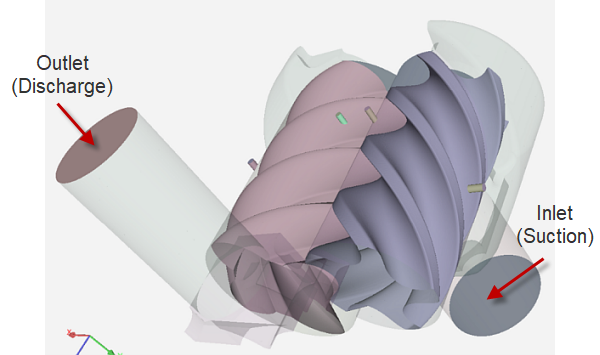
A screw compressor is a type of positive displacement compressor, which uses two spiral screws to compress the gas involved. The two spiral screws are a male rotor with convex blades and a female rotor with concave cavities which mesh together. Oil injection is often used in these compressors for sealing and cooling purposes, and we will examine the flows in an oil injected screw compressor in this tutorial. The project setup used in this tutorial is based on a realistic compressor studied by Rane et al.[2] The dimension and operating condition specifications are listed below:
Table 16.1: Dimensions and operating conditions of the example screw compressor
| Item | Value | Units |
|---|---|---|
| Working fluid | air (ideal gas) | - |
| Suction pressure | 1 | bar |
| Suction temperature | 298 | K |
| Discharge pressure | 8 | bar |
| Oil injection temperature | 323 | K |
| Male rotor rotation speed | 6000 | rev/min |
| Female rotor rotation speed | 4800 | rev/min |
| Number of lobes in male rotor | 4 | - |
| Number of lobes in female rotor | 5 | - |
Note: The directions of movement of the rotors are opposite, so a negative sign will be used for the Male Rotor’s angular velocity in the project.
The project setup workflow follows the top-down order of the workflow tree in the Ansys Forte Simulate interface. The components irrelevant to the present project will not be mentioned in this document, and you can simply skip them and use the default model options.
This simulation uses Forte’s on-the-fly automatic mesh generation (AMG) feature, which only requires the bounding surface geometry as an input and does not involve volume mesh generation ahead of the calculation. The surface geometry to be imported into Forte is in the (.stl) format in this tutorial. See the Geometry Import section in the Forte User's Guide for details.
Now let us import the surface geometry into the Forte Simulate user interface. Open
the Geometry panel, click the Import Geometry ![]() icon, select Surfaces from one or more STL files
as the import option, and select the provided STL file,
Screw_Compressor_Oil_Injected.stl. Accept all the default options on
the Import Options wizard window.
icon, select Surfaces from one or more STL files
as the import option, and select the provided STL file,
Screw_Compressor_Oil_Injected.stl. Accept all the default options on
the Import Options wizard window.
Forte's automatic mesh generation requires you to specify a material point, a global mesh size that serves as the reference size for mesh refinement, and various refinement controls.
Material Point: The Material Point ![]() should always lie inside the fluid domain throughout the simulation and
should be located at least one unit cell length away from any boundaries. In this tutorial
case, we choose to put the material point inside the Suction chamber: X = -3.0 cm,
Y = 18.0 cm, Z = -2.0 cm.
should always lie inside the fluid domain throughout the simulation and
should be located at least one unit cell length away from any boundaries. In this tutorial
case, we choose to put the material point inside the Suction chamber: X = -3.0 cm,
Y = 18.0 cm, Z = -2.0 cm.
Global Mesh Size: Set the Global Mesh Size to 0.4 cm.
Two types of refinement controls are used in this tutorial: Surface Refinement
Depth ![]() and Gap Feature Control
and Gap Feature Control ![]() . Surface Refinement Depth is used to refine meshes near wall boundaries
and open boundaries, while Gap Feature Control is used to refine meshes at the small
clearances (or “gaps”) between the rotors and the between the rotors and the
casing walls. Detailed mesh control parameters are listed in Table 16.2: Settings for Mesh Control refinements. The Active property is set to
Always for all the mesh controls. For the Gap Feature
Control, the Surface Proximity is set to 0.15
cm for the male and female casing sides and 0.1 for the
others and Enable Gap Model is turned ON.
. Surface Refinement Depth is used to refine meshes near wall boundaries
and open boundaries, while Gap Feature Control is used to refine meshes at the small
clearances (or “gaps”) between the rotors and the between the rotors and the
casing walls. Detailed mesh control parameters are listed in Table 16.2: Settings for Mesh Control refinements. The Active property is set to
Always for all the mesh controls. For the Gap Feature
Control, the Surface Proximity is set to 0.15
cm for the male and female casing sides and 0.1 for the
others and Enable Gap Model is turned ON.
Table 16.2: Settings for Mesh Control refinements
| Item | Refinement type | Refinement location | Refinement level | Refinement layers |
|---|---|---|---|---|
| Suction_Dischage_Chamber | Surface | discharge_pipe, discharge_port, suction_pipe, suction_port | 1/2 | 1 |
| Open_Boundaries | Surface | discharge_outlet, suction_inlet | 1/2 | 1 |
| Beam | Surface | suction_port_inner_beam | 1/4 | 1 |
| Casing_Side_Wall | Surface | casing_female_side, casing_male_side | 1/2 | 1 |
| Rotor_Side_Walls | Surface | female_rotor_side, male_rotor_side | 1/2 | 1 |
| Casing_End_Walls | Surface | casing_discharge_end,casing_suction_end | 1/4 | 1 |
| Rotor_End_Walls | Surface | female_rotor_discharge_end, female_rotor_suction_end, male_rotor_discharge_end, male_rotor_suction_end | 1/4 | 1 |
| Oil_Pipes | Surface | bottom_oil_pipe_1, bottom_oil_pipe_2, bottom_oil_pipe_3, side_oil_pipe | 1/4 | 1 |
| Oil_Inlets | Surface | bottom_oil_inlet_1, bottom_oil_inlet_2, bottom_oil_inlet_3, side_oil_inlet | 1/4 | 1 |
| Male_Casing_Side | Gap Feature | casing_male_side, male_rotor_side | 1/4 | |
| Female_Casing_Side | Gap Feature | casing_female_side, female_rotor_side | 1/4 | |
| Inter_Rotor | Gap Feature | female_rotor_side, male_rotor_side | 1/4 | |
| Male_Casing_Suction_End | Gap Feature | casing_suction_end, male_rotor_suction_end | 1/4 | |
| Male_Casing_Discharge_End | Gap Feature | casing_discharge_end, male_rotor_discharge_end | 1/4 | |
| Female_Casing_Suction_End | Gap Feature | casing_suction_end, female_rotor_suction_end | 1/4 | |
| Female_Casing_Discharge_End | Gap Feature | casing_discharge_end, female_rotor_discharge_end | 1/4 |
The Gap Feature Control ![]() is a mesh refinement control that is especially useful for handling the
small gaps in compressors. This control automatically detects small gaps between the
specified surface pair based on the user-specified Surface Proximity
criterion and applies refinement in the detected gap region based on the user-specified
refinement level. When Gap Feature Control is used, the spatially
resolved solution will contain a variable called GapCellFlag, which uses non-zero integer
values to mark the zones identified as gap zones.
is a mesh refinement control that is especially useful for handling the
small gaps in compressors. This control automatically detects small gaps between the
specified surface pair based on the user-specified Surface Proximity
criterion and applies refinement in the detected gap region based on the user-specified
refinement level. When Gap Feature Control is used, the spatially
resolved solution will contain a variable called GapCellFlag, which uses non-zero integer
values to mark the zones identified as gap zones.
Forte does not require the gap zones to be finely resolved using tiny CFD cells. In this tutorial, the Cartesian cell size in the gap zone is 0.1 cm, which means that some of the gaps only contain a fraction of a Cartesian cell cut by the physical boundary. To compensate for the under-resolution in the gap zones, the Gap Model is used to apply a momentum sink term, which accounts for the underpredicted wall shear stress and over-predicted mass flow rate on the coarse grid. The Gap Model takes both the gap size and the local fluid cell size as inputs, and therefore the flow solution is not expected to be very sensitive to the gap refinement level.
The Gap Size Scale Factor can be used to enlarge or shrink the gap sizes measured on the geometry. The scaled gap size is then used as the input for the gap model in each local CFD cell in the gap zone. If the gap size in the geometry accurately reflects the size in the actual compressor, the best practice is to use the default value of 1.0 and we have used this value in this tutorial. When using simulation to guide compressor design, this gap size scale factor also allows you to study the impact of gap size on simulation results without the need of modifying the geometry itself.
In Forte, a chemistry set in Chemkin format is used to define the properties of the
working fluid. This screw compressor involves two types of fluids. The main working fluid is
air, assumed to be a mixture of N2 and O2. It
will be modeled using the ideal gas model. Apart from air, oil will be injected via four
inlets for cooling and sealing purposes. To import gas species N2 and
O2, go to the Workflow tree and under Models
> Chemistry/Materials ![]() , click New Gas Species
, click New Gas Species ![]() , and add N2 and O2. To
import the oil, add a New Liquid and Vapour Pair
, and add N2 and O2. To
import the oil, add a New Liquid and Vapour Pair ![]() and add oil(l) and oil-vapor.
Under Liquid Properties, select User Defined
Values, then check the Override Database Liquid Density with Constant
Value box and use 800 kg/m3 as the density. Similarly, check
the Override Database Liquid Viscosity with Constant Value box and
use 0.0088 kg/m-sec as the viscosity. Also check the Override
Database Liquid Conductivity with Constant Value box and use 0.18
J/m-K-sec as the conductivity.
and add oil(l) and oil-vapor.
Under Liquid Properties, select User Defined
Values, then check the Override Database Liquid Density with Constant
Value box and use 800 kg/m3 as the density. Similarly, check
the Override Database Liquid Viscosity with Constant Value box and
use 0.0088 kg/m-sec as the viscosity. Also check the Override
Database Liquid Conductivity with Constant Value box and use 0.18
J/m-K-sec as the conductivity.
To define the main working fluid as air, click the Mixtures ![]() icon on the menu bar, and create a new gas mixture. In the Mixture
Editor window that displays, click Add Species to add
n2 and o2 and set the Mole
Fractions of o2 to
icon on the menu bar, and create a new gas mixture. In the Mixture
Editor window that displays, click Add Species to add
n2 and o2 and set the Mole
Fractions of o2 to 0.21 and that of
n2 to 0.79. Name this gas mixture as
“air_dry” for later use. To turn on the ideal gas model option, choose
Ideal Gas as the Equation of State option on the
Models > Chemistry/Materials panel.
Next, define a multiphase mixture in the mixture editor for oil injection. Add
oil(l) as the liquid phase species, and set the Liquid Phase
Fraction to 1.0. You can add any gas species to define the
gas phase, but since the Liquid Phase Fraction is 1.0, the effects of gas species are
trivial. Name this multiphase mixture as “oil” for later use.
The multiphase mixture will be used in boundary condition settings (see below) to specify oil injection. When the project has multiphase mixture defined in initial or boundary conditions, the Eulerian two-phase flow solver is automatically turned on. The Transport Model on the Chemistry/Materials panel determines which type of two-phase transport model is used. In this tutorial, the Volume Of Fluid is chosen due to its capabilities in tracking oil-air interface.
This tutorial uses the RANS RNG k-ε turbulence model, which is the default turbulence model option. Other turbulence modeling options are available under Models > Transport > Turbulence, such as LES models.
Use the icons on the Boundary Conditions panel to add new boundary conditions. The boundary conditions used in this project are explained below:
Suction_Inlet: Defined as an inlet boundary for air. For Composition on the inlet setup panel, select the air_dry mixture created earlier. Select surface suction_inlet as the Location. Choose the Total Pressure option for Inlet type and set the pressure to 1 bar. Change the Turbulent Kinetic Energy to 10,000 cm2/sec2 and Turbulent Length Scale to 1 cm. Choose Total Temperature as the Temperature Option and set the temperature to 298 K.
Static Walls: Next, we define boundary conditions for walls that do not move, namely, “static walls”. The static walls in this simulation include the following boundaries: Suction_Chamber, Discharge_chamber, Casing, and oil_pipes, as summarized in Table 16.3: Settings for static wall boundary conditions. Choose all the static walls as wall boundary and set the roughness height to 1 micron and roughness constant to 0.5. Keep the Wall Slip Condition as No Slip. The adiabatic wall boundary condition is assumed, so heat transfer is turned OFF for all the walls (static and moving).
Table 16.3: Settings for static wall boundary conditions
| Boundary name | Location |
|---|---|
| Suction_Chamber | suction_pipe, suction_port, suction_port_inner_beam |
| Discharge_Chamber | discharge_pipe, discharge_port |
| Casing | casing_discharge_end, casing_female_side, casing_male_side, casing_suction_end |
| Oil_pipes | bottom_oil_pipe_1, bottom_oil_pipe_2, bottom_oil_pipe_3, side_oil_pipe |
Moving Walls: The moving walls in this simulation include the rotors, namely, the Male_Rotor and Female_Rotor boundaries. Keep the settings the same as the static walls, unless specified otherwise. Enable Wall Motion, set Motion Type to Rotation and set Movement Type to Moving Surface. To set up the rotational motion, you must define the origin and direction of the rotation axis. For this purpose, it is convenient to define two reference frames for the male and female rotors. From the Geometry node, select Reference Frames and create the following two new reference frames: Male_Rotor_Axis and Female_Rotor_Axis. For reference frame Male_Rotor_Axis, set the New Origin to (X = 1.418 cm, Y = -0.354 cm, Z = -7.8 cm); for reference frame Female_Rotor_Axis, set the New Origin to (X = -7.882 cm, Y = -0.354 cm, Z = -7.8 cm). Then, the Axis Origin is set as the origin of the relevant reference frame, while the Axis Direction is set as the z-direction. The two moving wall boundary conditions’ locations, reference frames, and angular velocities of rotation are summarized in Table 16.4: Settings for moving wall boundary conditions.
Table 16.4: Settings for moving wall boundary conditions
| Boundary name | Location | Reference frame | Angular velocity (rpm) |
| Male_Rotor | male_rotor_discharge_end, male_rotor_side, male_rotor_suction_end | Male_Rotor_Axis | -6000 |
| Female_Rotor | female_rotor_discharge_end, female_rotor_side, female_rotor_suction end | Female_Rotor_Axis | 4800 |
Oil Inlets: There are four oil inlets in the geometry, defined as
inlet boundary ![]() . For all four inlets, set the inlet fluid’s composition as the
multiphase mixture oil described in Chemistry Setup and the Inlet as Mass
Flow Rate. Change the Inflow Mixture Density Option to
Specify Static Density with the Density set to
0.8 gm/cm3. Keep the Turbulence parameters the
same as for Suction_Inlet and use a Static
Temperature of 323 K as the Temperature
Option. Table 16.5: Settings for oil inlets' boundary conditions summarizes the mass flow
rates specified for each oil inlet.
. For all four inlets, set the inlet fluid’s composition as the
multiphase mixture oil described in Chemistry Setup and the Inlet as Mass
Flow Rate. Change the Inflow Mixture Density Option to
Specify Static Density with the Density set to
0.8 gm/cm3. Keep the Turbulence parameters the
same as for Suction_Inlet and use a Static
Temperature of 323 K as the Temperature
Option. Table 16.5: Settings for oil inlets' boundary conditions summarizes the mass flow
rates specified for each oil inlet.
Table 16.5: Settings for oil inlets' boundary conditions
| Boundary name | Location | Mass Flow Rate (g/sec) |
|---|---|---|
| Oil_inlet_1 | bottom_oil_inlet_1 | 600 |
| Oil_inlet_2 | bottom_oil_inlet_2 | 550 |
| Oil_inlet_3 | bottom_oil_inlet_3 | 1100 |
| Oil_inlet_4 | side_oil_inlet_1 | 900 |
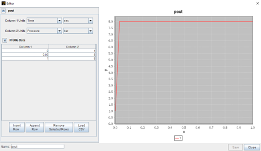
Discharge_outlet: This is defined as an outlet boundary for both air and oil, but defined as an inlet type, with the surface discharge_outlet specified as the Location. The decision to specify the outlet as an inlet boundary allows specifying a temperature at the outlet, which is helpful when reverse flow happens. The nominal outlet pressure is 8 bar. However, instead of setting a constant pressure at the outlet, we recommend setting the Total Pressure, Time Varying condition for the Inlet and creating a pressure profile at the inlet that ramps up the pressure from 1 to 8 bar and maintains it for the length of the simulation. Ramping up outlet pressure in the early stage of simulation helps with stability in the flow solver. To do this, select Create new… under Pressure Profile, name it p_out and use the pressure profile as illustrated in Figure 16.2: Outlet pressure profile for screw compressor:
Uncheck the Treat Profile as Cyclic check box. Keep the Turbulence parameters the same as for Suction_Inlet and use a Static Temperature of 340 K as the Temperature Option. The fluid Composition is set as air_dry, with the assumption that only air but no oil exists in the reverse flow.
For Composition, select the mixture air_dry, which was created earlier. Set Temperature to 298 K and Pressure to 1 bar.
Simulation Limits: Select the Time Based option to specify the Simulation End Point and set Max. Simulation Time to 0.12 sec. This duration covers 12 complete revolutions for the male rotor. (The time for each resolution can be calculated as 60/RPM s).
Time Step: Forte uses adaptive time step controls to adjust the actual time step size for each transient flow integration step. The user-specified maximum time step will be used if the time step is not subject to other constraints listed under Advanced Time Step Control Options. For rotating machinery simulations, the rule of thumb for choosing the Maximum Simulation Time Step is to have at least 10 time steps per degree of rotation of the fastest rotating motion in the system. Using this guideline, the Max Time Step can be estimated as 60/(RPM*360*10) = 1/(RPM*60) sec, which gives 3E -6 s for RPM = 6000. In this tutorial, the Max Time Step is set to 3.0E-6 s. For the Advanced Time Step Control Options, typically it is acceptable to relax the Fluid Acceleration Factor and Rate of Strain Factor to achieve larger time steps without affecting the accuracy and stability excessively. In this calculation, these two factors are set to the recommended values of 0.5 and 0.6, respectively. It is risky to change the other control factors because relaxing them may cause the solution to become unstable.
Chemistry Solver: Set the Activate Chemistry option to Always Off because this simulation does not involve chemical reactions.
Spatially Resolved: Set the Output Timing Control as Time. Set Interval Based Output Control to output every 0.001 s, which corresponds to 1/10 of a full revolution. For the Solution Variables list, select variables of interest. The minimum variable set should include Pressure, Temperature, VelocityX, VelocityY, VelocityZ, and Velocity Magnitude.
Spatially Averaged And Spray: Choose the Spatially Averaged Output Control option as Time and set the output interval to 1.0E-4 s. Select species n2 and o2 for output.
Restart Data: Make sure Write Restart File at Last Simulation Step is checked ON. This option allows a restart file to be saved at the end of the current simulation. Such a restart file is useful if you decide to extend the simulation duration to do parameter studies because it provides a much better guess for initial conditions than uniform initial conditions would. This practice may help save CPU time spent in simulating the initial transient process. Turn ON Interval Based Restart and set the Time Steps between Restart Writing to 1000. This type of restart file can help provide a recovery point if a long-running job was unexpectedly interrupted.
The Preview Simulation utility is a useful tool for checking boundary
motion, detecting potential surface intersection and verifying volume mesh generation ahead of
the calculation. Open the Mesh Generation panel under Preview
Simulation, select Time Range as the Time
Option, set the Start, End, and Step to
0.0 s, 0.12 s, 0.01 s, respectively. Since one complete revolution takes
0.01 s at 6000 RPM, this preview schedule will produce 12 snapshots within a revolution. Click
the Generate Mesh ![]() icon on the panel, then select PreviewData.dvs and
click OK on the dialog that displays. Ansys EnSight will be launched
automatically and the preview solutions will be gradually loaded in EnSight as soon as they
are created.
icon on the panel, then select PreviewData.dvs and
click OK on the dialog that displays. Ansys EnSight will be launched
automatically and the preview solutions will be gradually loaded in EnSight as soon as they
are created.
By default, the Check for Surface Intersections and Include Volume Mesh boxes are not selected, and the preview is only for checking surface mesh motion. This type of preview is very fast to process. You can run this preview in serial mode and create dozens of snapshots. The preview solution should be produced almost instantly in EnSight.
If Check for Surface Intersections is turned ON, the preview requires slightly longer CPU time. A new Part called intersections will be added to the part list in EnSight. If any surface intersection occurs, the surface triangles involved in the intersections will show up in this new Part.
If Include Volume Mesh is turned ON, the volume mesh preview results will take a considerably longer CPU time to produce. We recommend running the volume mesh preview in MPI mode and limiting the preview locations to a few snapshots. Doing a snapshot check for the volume mesh is valuable for detecting setup errors in the material point and the surface normal and also for verifying mesh refinement settings.
The run settings depend on the system and environment for your simulations. All the default options are appropriate for running this tutorial. The only thing to customize is the number of MPI processes used to run the job. The default value is 16, but it can be modified under Run Settings > Run Options > Job Script Options > Default MPI Arguments. The actual value used in the run can be further modified on the Run Simulation panel, shown as MPI Arguments. The CPU time needed to run this case is described in Time Estimate. If possible, use more MPI cores to shorten the turnaround time. Refer to the Forte User's Guide if you need to set up multiple runs in a parameter study.
This section discusses using the output to visualize and post-process results:
The spatially averaged solutions are reported in CSV format in the Run folder (Nominal).
Ansys Forte Monitor ![]() is a convenient tool for displaying these averaged solutions. Launch
Forte Monitor and open the analysis directory of the Forte
project to load the CSV files. The parameters plotted show the accumulated mass flow rate at
the Inlet (open_boundary_flow.csv). In this example, the
curves show that the simulation has largely reached a steady operation since the accumulated
mass flow rate has stabilized around a constant value.
is a convenient tool for displaying these averaged solutions. Launch
Forte Monitor and open the analysis directory of the Forte
project to load the CSV files. The parameters plotted show the accumulated mass flow rate at
the Inlet (open_boundary_flow.csv). In this example, the
curves show that the simulation has largely reached a steady operation since the accumulated
mass flow rate has stabilized around a constant value.
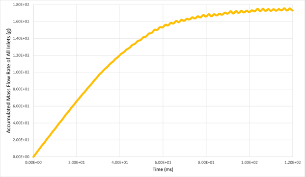
Once a steady operation is observed from the simulation results, one can study the inflow and outflow rate of air and oil and check if they are reasonable or not. It can be seen from Figure 16.3: Accumulated mass flow rate at inlet that the steady operation is reached after around 120 msec, or 12 revolutions of the male rotor. This is why we have set the simulation duration to this number.
Ansys EnSight is the preferred tool for visualizing the spatially resolved solutions. Launch EnSight and open the .ftind file to load the solutions. The .ftind file is a solution index file, which contains the records pointing to a group of .ftres files. The actual solution data are contained in the .ftres files. If you need to control which .ftres solution(s) to load in EnSight, you can truncate or concatenate the records contained in the .ftind files in a text editor. Refer to the Forte User's Guide for details.
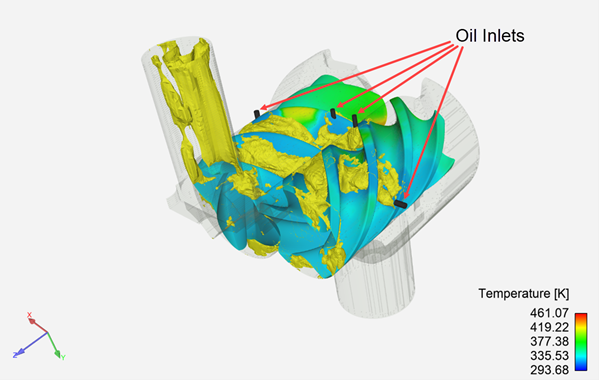
On the EnSight Part tree shown, the Part VolumeCells is the one that contains the 3-D volume solutions. It can be used for creating clip planes, isosurfaces, particle traces, and more. Figure 16.4: Isosurfaces of oil volume fraction = 0.1 using EnSight shows the isosurfaces of the oil volume fraction = 0.1, colored yellow, and the male and female rotors, colored by temperature.
[2] Rane, S. R.; Kovacevic, A.; and Stosic, N., "CFD Analysis of Oil Flooded Twin Screw Compressors" (2016). International Compressor Engineering Conference. Paper 2392.