This tutorial describes how to use Ansys Forte CFD to simulate the gas flow in a rotary lobe compressor. A blower case is used in this tutorial as an example, but the simulation methodology, conventions, and best practices also apply to all other types of rotary lobe compressors that involve two engaging rotors, such as screw compressors and gear compressors. The geometry used in this tutorial represents a non-proprietary, generic rotary lobe compressor. It is used only for demonstrating the simulation setup using Forte and should not be used as a guidance for actual machine design.
This tutorial first explains the methodology and conventions used in compressor simulation, and then goes through all the simulation setup steps, with emphasis on the following aspects that are unique or important to compressors:
Requirements for surface geometry preparation
Small gap handling using gap refinement controls and gap model
Rotational motion setup
Simulation preview for checking boundary motion and potential surface intersection
Visualization of simulation results
The following sections describe the provided files, time required, prerequisites, and a utility for comparing your generated project file (.ftsim) with the one provided in the tutorial download.
This tutorial will cover all the set-up steps, but we recommend that you work through the Forte Quick Start Guide first and become familiar with the workflow of the Ansys Forte user interface.
The files for this tutorial are obtained by downloading the
lobe_compressor.zip file
here
.
Unzip lobe_compressor.zip to your working folder.
Files provided in this tutorial include a Forte project file that has been fully configured as well as a set of facilitating input files that can be used to set up the Forte project from scratch. Specifically, the files include:
Rotary_Lobe_Compressor_Tutorial.ftsim: The fully configured Forte project file.
Rotary_Lobe_Compressor_Surface_Geometry.tgf: Surface geometry input file in Fluent Meshing faceted geometry (.tgf) format, which was exported from SpaceClaim.
Air_NoReactions_chem.inp: Chemistry input file in Ansys Chemkin format, which is used to set up the working fluid properties in Forte simulation.
The tutorial sample compressed archive is provided as a download. You have the opportunity to select the location for the file when you download and uncompress the sample files.
Note: This tutorial is based on a fully configured sample project that contains the tutorial project settings. The description provided here covers the key points of the project set-up but is not intended to explain every parameter setting in the project. The project files have all custom and default parameters already configured; the text highlights only the significant points of the tutorial.
Forte may be launched in a command line mode to perform certain tasks such as preparing a run for execution, importing project settings from a text file, or various other tasks described in the Forte User's Guide. One of these tools allows exporting a textual representation of the project data to a text file.
Example
forte.sh CLI -project <project_name>.ftsim -export tutorial_settings.txt
Briefly, you can double-check project settings by saving your project and then running the command-line utility to export the settings in your tutorial project (<project_name>.ftsim), and then use the command a second time to export the settings in the provided final version of the tutorial. Compare them with your favorite diff tool, such as DIFFzilla. If all the parameters are in agreement, you have set up the project successfully. If there are differences, you can go back into the tutorial set-up, re-read the tutorial instructions, and change the setting of interest.
This Forte project is set up to run for five complete revolutions. As a guideline for your own simulations, this tutorial is estimated to take approximately 19 hours on a Linux cluster using an Intel 2.6 GHz processor (168 cores). Another test run on a Windows PC using 20 cores took approximately 75 hours.
The geometry and working principle of the sample blower are illustrated in Figure 13.1: Configuration of the sample blower case. Two engaging three-lobed rotors rotate within a casing. These two rotors rotate at the same rotational speed, but around opposite directions. The rotation directions are shown by the curved arrows. The rotors' rotation motion causes the working fluid (air in this case) to be sucked into the casing through the suction inlet. As the working fluid travels through the compartments formed between the rotor surfaces and the casing surfaces, it is compressed and eventually discharged through the discharge outlet with raised temperature and pressure. One of the rotors is driven by an electric motor, and the shafts of these two rotors engage through helical gears outside of the casing. The two rotors do not have direct surface contact. The dimension and operating condition specifications are listed in Table 13.1: Dimensions and operating conditions of the sample blower.
Table 13.1: Dimensions and operating conditions of the sample blower
| Item | Value | Units |
|---|---|---|
| Rotor diameter | 16 | cm |
| Rotor length | 20 | cm |
| Helical pitch of the rotors | 300 | cm |
| Distance between rotors' axes | 12 | cm |
| Working fluid | air (ideal gas) | |
| Suction pressure (Total) | 1 | bar |
| Suction temperature (Total) | 300 | K |
| Discharge pressure (Total) | 3 | bar |
| Discharge temperature (Total) | 375 | K |
| Rotation Speed | 6000 | rev/min |
The project setup workflow follows the top-down order of the workflow tree in the Ansys Forte Simulate interface. The components irrelevant to the present project will not be mentioned in this document, and you can simply skip them and use the default model options.
This simulation uses Forte's on-the-fly automatic mesh generation (AMG) feature, which only requires the bounding surface geometry as an input and does not involve volume mesh generation ahead of the calculation. The surface geometry to be imported into Forte is in Fluent Meshing faceted geometry (.tgf) format, which was exported from the solid geometry created in SpaceClaim. Although the TGF format is used in this tutorial, several other formats are also allowed. See the Geometry Import section in the Forte User's Guide for details.
Since the rotors in compressors involve curved surfaces in 3-D and there are tiny gaps between the rotors and the casing and also between the two rotors, the curved surfaces are required to be sufficiently smooth in order to avoid surface intersection during the rotation. When exporting the TGF file from SpaceClaim, we recommend that you choose the Fine option for the Facet Resolution of the TGF file. The Angle resolution should not be much larger than 4°.
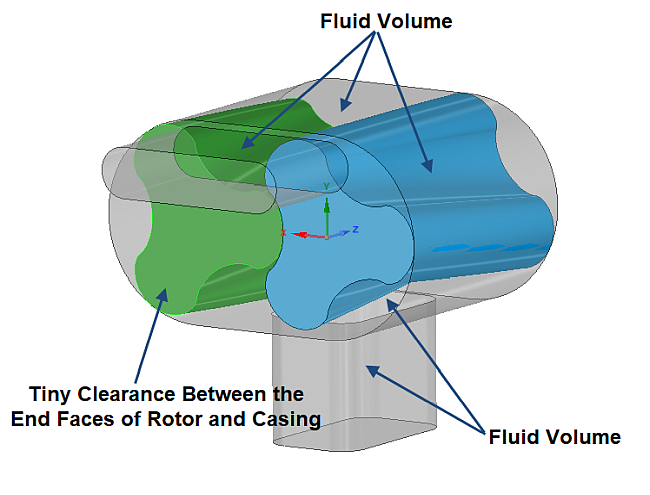
The fluid domain in this case is formed by three watertight surface groups. The first group consists of the inlet, outlet, suction and discharge port walls, and the casing wall (Part a, Figure 13.2: Surface normal vectors of the casing and rotors), the other two groups are for the two rotors, each consisting of two end surfaces and one side surface (Part b, Figure 13.2: Surface normal vectors of the casing and rotors). Fluid volume is formed between the exterior of the rotor solids and the interior of the "casing + ports" solid (shown in Figure 13.3: Fluid volume formation between casing and rotors). Forte requires that the end surfaces of the rotors be put inside the casing and away from the casing's end surfaces by a tiny tolerance. In the provided geometry file, this tiny tolerance is 1 µm. By default, the gap between the rotor end surface and the casing end surface will not be meshed in the volume mesh. However, if the end gap sizes are physically large enough and it is desirable to model the flow leakage through them, we can force these gaps to be meshed by using the gap refinement controls that will be discussed later in the Automatic Mesh Generation Setup section.
In Forte, the normal vectors of the triangulated surface mesh are required to point towards the exterior of the fluid domain. The surface normals of the casing and rotors are illustrated by the red arrows in Figure 13.2: Surface normal vectors of the casing and rotors. When the solids of the casing and rotors are created in SpaceClaim, the normals are assumed to point to the interior of the solids. Therefore, after a TGF or STL file exported from SpaceClaim is imported into Forte, the normals of the Casing surfaces (as well as the inlet/outlet and suction/discharge port walls) should be inverted.
Tip:
An incorrect (flipped) surface normal is one of the most common reasons for meshing errors. The surface normals should be carefully checked after the geometry import.
When preparing the geometry in SpaceClaim, use Named Groups to group the boundary surfaces and give each group a name. When a geometry with Named Groups is imported in Forte, Forte will use the same naming convention. Therefore, you can avoid the requirement to split the surface geometry inside the Forte user interface. Doing so also makes it convenient to replace the geometry if needed. When an updated geometry using the same Named Groups is imported, the old surfaces will be automatically replaced at all the places where these surfaces are used, such as in refinement controls and boundary conditions. Notice that you may still need to invert the normals for some of the newly imported surfaces based on the requirements described above.
Now let us import the surface geometry into the Forte Simulate user interface. Open
the Geometry panel, click the Import Geometry ![]() icon, select Surfaces from TGF file as the import
option, and select the provided TGF file,
Rotary_Lobe_Compressor_Surface_Geometry.tgf. Accept all the default
options on the Import Options wizard window. Ensure that the
Invert Normals box is checked, so that the normals of the imported
surfaces will point to the exterior of the solids, and consequently you should invert the
normals back for the rotor surfaces after the import. In the Workflow tree under the
Geometry node, multi-select (hold Ctrl while clicking) surfaces
left_rotor_discharge_end, left_rotor_side,
left_rotor_suction_end, right_rotor_discharge_end,
right_rotor_side, right_rotor_suction_end, and on
the right-click menu, choose Invert Normals. You can double-check the
normals of a surface by turning on Normals on this right-click menu.
icon, select Surfaces from TGF file as the import
option, and select the provided TGF file,
Rotary_Lobe_Compressor_Surface_Geometry.tgf. Accept all the default
options on the Import Options wizard window. Ensure that the
Invert Normals box is checked, so that the normals of the imported
surfaces will point to the exterior of the solids, and consequently you should invert the
normals back for the rotor surfaces after the import. In the Workflow tree under the
Geometry node, multi-select (hold Ctrl while clicking) surfaces
left_rotor_discharge_end, left_rotor_side,
left_rotor_suction_end, right_rotor_discharge_end,
right_rotor_side, right_rotor_suction_end, and on
the right-click menu, choose Invert Normals. You can double-check the
normals of a surface by turning on Normals on this right-click menu.
To facilitate the subsequent setup steps, we now define two Reference
Frames, one for each rotor. Go to Geometry >
Reference Frames, click the New Reference Frame ![]() icon to create these two reference frames. Refer to the fully
configured .ftsim file for details. Reference frame
RF_Right_Rotor is the same as the global origin, and
RF_Left_Rotor has its origin moved to X = 12.0 cm
relative to the global origin. In this way, the origin of each reference frame anchors the
center of the suction end face of the rotor, and the Z-axis aligns with the rotor's
rotating axis.
icon to create these two reference frames. Refer to the fully
configured .ftsim file for details. Reference frame
RF_Right_Rotor is the same as the global origin, and
RF_Left_Rotor has its origin moved to X = 12.0 cm
relative to the global origin. In this way, the origin of each reference frame anchors the
center of the suction end face of the rotor, and the Z-axis aligns with the rotor's
rotating axis.
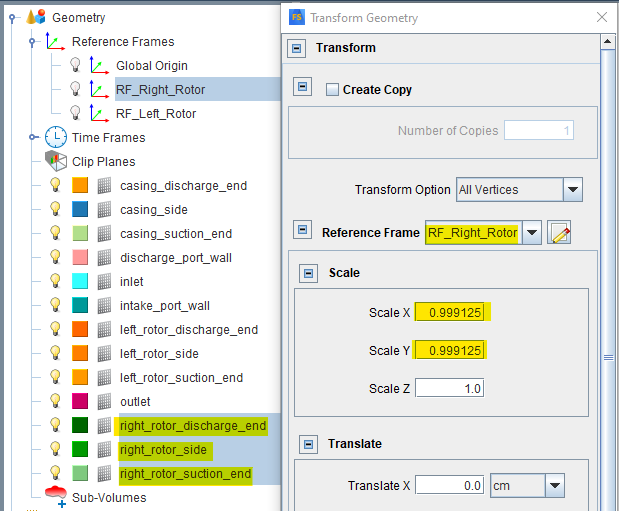
When the geometry used in this tutorial was created in SpaceClaim, there are zero rotor-casing or rotor-rotor gaps. We will create a 70 µm (0.007 cm) gap between the rotors and the casing by shrinking the rotors slightly along their radial direction. Since the maximum radius of the rotor is 8.0 cm, the shrinking factor is 1-0.007/8.0 = 0.999125. An example using the right rotor is shown in Figure 13.4: Use Transform Mesh to shrink the rotors along the radial direction. Select the three surfaces corresponding to the right rotor, select Transform Mesh on the right-click menu, choose the Reference Frame named RF_Right_Rotor created earlier and scale X and Y by 0.999125. Repeat the same procedure for the left rotor using Reference Frame named RF_Left_Rotor. Using the method of shrinking the rotors to create gaps, the gaps between the rotors and the casing are well controlled and the smallest distance is 70 µm. However, the gap sizes between the two rotors vary both temporally and spatially, and the inter-rotor gap sizes at the engaging locations could be much smaller than 70 µm.
Automatic mesh generation in Forte requires you to specify a material point, a global mesh size that serves as the reference size for mesh refinement, and various refinement controls.
Material Point: The material point should always lie inside the fluid domain throughout the simulation and should be located at least one unit cell length away from any boundaries. In this tutorial case, we choose to put the material point inside the suction port: X = 6.0 cm, Y = 5.0 cm, Z = -5.0 cm.
Global Mesh Size: Set the Global Mesh Size to 0.4 cm.
Three types of refinement controls are used in this tutorial: Surface Refinement Depth, SAM (Solution Adaptive Mesh), and Gap Feature Control. Detailed mesh control parameters are listed in Table 13.2: Settings for Mesh Control refinements. The Active property is set to Always for all the mesh controls. For the three Gap Feature Controls, the Surface Proximity is set to 0.15 cm, and Enable Gap Model is turned ON.
Tip: Material Point being outside of the fluid domain is another commonly encountered setup error, which causes meshing failure. Make sure the Material Point will not go out of the domain due to boundary motion.
Table 13.2: Settings for Mesh Control refinements
| Item | Refinement type | Refinement location | Refinement level | Refinement layers |
|---|---|---|---|---|
| Side_Walls | Surface | casing_side, discharge_port_wall, intake_port_wall, left_rotor_side, right_rotor_side | 1/2 | 1 |
| End_Walls | Surface | casing_discharge_end, casing_suction_end, left_rotor_discharge_end, left_rotor_suction_end, right_rotor_discharge_end, right_rotor_suction_end | 1/4 | 1 |
| Open_Boundaries | Surface | inlet, outlet | 1/2 | 1 |
| SAM_Velocity_Grad | SAM Quantity Type = Gradient of Solution Field; Solution Variables = VelocityMagnitude; Bounds = Statistical; Sigma Threshold = 0.5 | Entire Domain | 1/2 | |
| Left_Rotor_Casing | Gap Feature | (casing_side, left_rotor_side) | 1/4 | |
| Right_Rotor_Casing | Gap Feature | (casing_side, right_rotor_side) | 1/4 | |
| Inter_Rotor | Gap Feature | (left_rotor_side, right_rotor_side) | 1/4 |
The Gap Feature Control is a mesh refinement control that is especially useful for handling the small gaps in compressors. This control automatically detects small gaps between the specified surface pair based on the user-specified Surface Proximity criterion and applies refinement in the detected gap region based on the user-specified refinement level. When Gap Feature Control is used, the spatially resolved solution will contain a variable called GapCellFlag, which uses non-zero integer values to mark the zones identified as gap zones.
Forte does not require the gap zones to be finely resolved using tiny CFD cells. In this tutorial, the Cartesian cell size in the gap zone is 0.1 cm, which means that some of the gaps only contain a fraction of a Cartesian cell cut by the physical boundary. To compensate for the under-resolution in the gap zones, the Gap Model is used to apply a momentum sink term, which accounts for the underpredicted wall shear stress and over-predicted mass flow rate on the coarse grid. The Gap Model takes both the gap size and the local fluid cell size as inputs, and therefore the flow solution is not expected to be very sensitive to the gap refinement level.
As mentioned earlier, there is a 1 µm distance tolerance between the end surface of the rotor and the end surface of the casing on both ends. Forte will ignore this tiny gap by default. However, if the end gaps are large enough and it is of interest to model the flow leakage through them, you can use the Gap Feature Control to mesh these gaps.
In Forte, a chemistry set in Chemkin format is used to define the properties of the working fluid. The chemistry input file used in this tutorial contains air (O2 and N2) and no reactions. In the provided chemistry input file, Air_NoReactions_chem.inp, species o2 is duplicated as o2_in, o2_out, and n2 is duplicated as n2_in and n2_out, respectively. By doing this, we can use the _in version to define the inflow mixture and use the _out version to define the reverse flow mixture. The original o2 and n2 are used to define the initial mixture inside the domain. Such a setup allows us to track how the initial mixture is flushed out of the domain during the initial transient process and how the inflow and reverse flow mixtures are distributed inside the domain under steady state operation.
Now let us create a chemistry set using Air_NoReactions_chem.inp
and import it into Forte. Under Utility on the ribbon or menu bar,
click the PreProcess icon, and follow the wizard to create a
New Chemistry Set: Select Air_NoReactions_chem.inp
as the Gas-Phase Kinetics File. Then go back to the setup Workflow
tree: Models > Chemistry/Materials, click the
New Import Chemistry ![]() icon to open the new chemistry set (.cks) file we
just created.
icon to open the new chemistry set (.cks) file we
just created.
Forte has both ideal gas and real gas model options. To turn on the ideal gas model option, choose Real Gas as the Equation of State option on the Models > Chemistry panel. In this tutorial, we will keep the default Ideal Gas option.
This tutorial uses the RANS RNG k-epsilon turbulence model, which is the default turbulence model option. Other turbulence modeling options are available under Models > Transport > Turbulence, such as LES models.
Use the icons on the Boundary Conditions panel to add new boundary conditions. The boundary conditions used in this project are explained below:
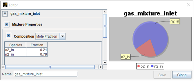
Suction_Inlet: Defined as an inlet boundary ![]() . For Composition on the inlet setup panel, select
Create new gas mixture... to create a mixture called
gas_mixture_inlet using species o2_in and n2_in (Figure 13.5: Example for setting up a new gas mixture). Select surface inlet as the
Location. Choose the Total Pressure option for
Inlet type and set the pressure to 1.0 bar. Keep
the default turbulence parameters for the inflow. Choose Total
Temperature as the Temperature Option and set the
temperature to 300 K.
. For Composition on the inlet setup panel, select
Create new gas mixture... to create a mixture called
gas_mixture_inlet using species o2_in and n2_in (Figure 13.5: Example for setting up a new gas mixture). Select surface inlet as the
Location. Choose the Total Pressure option for
Inlet type and set the pressure to 1.0 bar. Keep
the default turbulence parameters for the inflow. Choose Total
Temperature as the Temperature Option and set the
temperature to 300 K.
Discharge_Outlet: The discharge outlet should be defined as an
inlet boundary ![]() as well because we need the reverse flow condition to be explicitly
defined. For Composition, create a new mixture called
gas_mixture_outlet using species o2_out and n2_out (similar to the
one shown in Figure 13.5: Example for setting up a new gas mixture). Select the surface named
outlet as the Location. Choose the
Total Pressure option for Inlet type and set the pressure
to 3.0 bar. Keep the default turbulence parameters for the inflow.
Choose Total Temperature as the Temperature Option
and set the temperature to 375 K.
as well because we need the reverse flow condition to be explicitly
defined. For Composition, create a new mixture called
gas_mixture_outlet using species o2_out and n2_out (similar to the
one shown in Figure 13.5: Example for setting up a new gas mixture). Select the surface named
outlet as the Location. Choose the
Total Pressure option for Inlet type and set the pressure
to 3.0 bar. Keep the default turbulence parameters for the inflow.
Choose Total Temperature as the Temperature Option
and set the temperature to 375 K.
Suction_Port: Defined as a wall boundary ![]() . Select surface intake_port_wall as the
Location. Turn on Heat Transfer and set
Wall Temperature to 300.0 K, which is the same as
the inflow temperature at Suction_Inlet.
. Select surface intake_port_wall as the
Location. Turn on Heat Transfer and set
Wall Temperature to 300.0 K, which is the same as
the inflow temperature at Suction_Inlet.
Discharge_Port: Defined as a wall boundary ![]() . Select surface discharge_port_wall as the
Location. Turn on Heat Transfer and set
Wall Temperature to 375.0 K, which is the same as
the reverse flow temperature at Discharge_Outlet.
. Select surface discharge_port_wall as the
Location. Turn on Heat Transfer and set
Wall Temperature to 375.0 K, which is the same as
the reverse flow temperature at Discharge_Outlet.
Casing: Defined as a wall boundary ![]() . Select surfaces casing_discharge_end,
casing_side, and casing_suction_end as the
Location. Turn on Heat Transfer and set
Wall Temperature to 320.0 K. You can also use
the spatially varying wall temperature option to set up a boundary condition look-up table
to vary the temperature along the axial direction of the casing.
. Select surfaces casing_discharge_end,
casing_side, and casing_suction_end as the
Location. Turn on Heat Transfer and set
Wall Temperature to 320.0 K. You can also use
the spatially varying wall temperature option to set up a boundary condition look-up table
to vary the temperature along the axial direction of the casing.
Right_Rotor: Defined as a wall boundary ![]() with wall motion. Select surfaces
right_rotor_discharge_end, right_rotor_side, and
right_rotor_suction_end as the Location. Turn off
Heat Transfer to model the rotor wall as adiabatic. Turn on
Wall Motion and set Motion Type as
Rotation. The rotation axis requires an Origin and a
Direction vector as the inputs. Although they can be specified in an
arbitrary way, with respect to any Reference Frame, it is more convenient to take advantage
of the Reference Frames we created earlier for each rotor. For the right rotor, if the
Reference Frame named RF_Right_Rotor is used, the
Origin and Direction of the rotation axis are
simply the origin (X = 0.0 cm, Y = 0.0 cm, Z = 0.0 cm) and Z-axis
(X = 0.0, Y = 0.0, Z = 1.0) of this reference frame. Set
Angular Velocity to 6,000 RPM. Note that the
rotation direction follows the right-hand rule.
with wall motion. Select surfaces
right_rotor_discharge_end, right_rotor_side, and
right_rotor_suction_end as the Location. Turn off
Heat Transfer to model the rotor wall as adiabatic. Turn on
Wall Motion and set Motion Type as
Rotation. The rotation axis requires an Origin and a
Direction vector as the inputs. Although they can be specified in an
arbitrary way, with respect to any Reference Frame, it is more convenient to take advantage
of the Reference Frames we created earlier for each rotor. For the right rotor, if the
Reference Frame named RF_Right_Rotor is used, the
Origin and Direction of the rotation axis are
simply the origin (X = 0.0 cm, Y = 0.0 cm, Z = 0.0 cm) and Z-axis
(X = 0.0, Y = 0.0, Z = 1.0) of this reference frame. Set
Angular Velocity to 6,000 RPM. Note that the
rotation direction follows the right-hand rule.
Left_Rotor: Defined as a wall boundary ![]() with wall motion. Select surfaces
left_rotor_discharge_end, left_rotor_side,
left_rotor_suction_end as the Location. Use the
same Heat Transfer and Wall Motion settings as the
Right_Rotor, except that it should use the Reference
Frame named RF_Left_Rotor instead. Set Angular
Velocity to -6,000 RPM to let it rotate in the opposite
direction as the Right_Rotor wall.
with wall motion. Select surfaces
left_rotor_discharge_end, left_rotor_side,
left_rotor_suction_end as the Location. Use the
same Heat Transfer and Wall Motion settings as the
Right_Rotor, except that it should use the Reference
Frame named RF_Left_Rotor instead. Set Angular
Velocity to -6,000 RPM to let it rotate in the opposite
direction as the Right_Rotor wall.
Note: In this blower example, since the two rotors have the same number of lobes (gear ratio = 1), they have the same angular velocity magnitude and rotate along opposite directions. In a screw compressor, the ratio of the angular velocities of the male and female rotors is proportional to the reciprocal of their gear ratio.
For Composition, create a new gas mixture called gas_mixture_initial using species o2 and n2, similar to the one shown in Figure 13.5: Example for setting up a new gas mixture. Set Temperature to 300 K and Pressure to 1.0 bar. It is not critical to have well guessed initial conditions because the initial mixture can be quickly flushed out and overridden by steady operation conditions after 2 to 3 revolutions.
Simulation Limits: Choose the Time Based option to specify the Simulation End Point and set Max. Simulation Time to 0.05 s. This duration covers five complete revolutions for each rotor at 6000 RPM (Time for each revolution can be calculated as 60/RPM s).
Time Step: Forte uses adaptive time step controls to adjust the actual time step size for each transient flow integration step. The user-specified max time step will be used if the time step is not subject to other constraints listed under Advanced Time Step Control Options. For rotating machinery simulation, the rule of thumb for choosing the Max. Simulation Time Step is to have at least 10 time steps per degree of rotation of the fastest rotating motion in the system. Using this guideline, the Max Time Step can be estimated as 60/(RPM*360*10) = 1/(RPM*60) s, which gives 2.78E-6 s for RPM = 6000. In this tutorial, the Max Time Step is set to 2.5E-6 s. For the Advanced Time Step Control Options, typically it is acceptable to relax the Fluid Acceleration Factor and Rate of Strain Factor to achieve larger time steps without affecting the accuracy and stability very much. In this calculation, these two factors are set to 1.0 and 1.2, respectively. Both are two times their default values. It is risky to change the other control factors because relaxing them may cause the solution to become unstable.
Chemistry Solver: Set the Activate Chemistry option to Always Off because this simulation does not involve chemical kinetics.
Spatially Resolved: Use Time as the Output Timing Control option. Set Interval Based Output Control to output every 0.01 s, which corresponds to one revolution. Turn on User Defined Output Controls and create a time list to save spatially-resolved solutions at locations of interest. In the fully configured .ftsim file, the solutions are saved for every 0.001 s for the first revolution and the fifth revolution. For the Spatially Resolved Species list, select all the species. For the Solution Variables list, select variables of interest. The minimum variable set should include Pressure, Temperature, VelocityX, VelocityY, VelocityZ, and VelocityMagnitude.
Spatially Averaged And Spray: Choose the Time option and set the output interval to 1.0E-5 s. Select all the species for output.
Restart Data: Make sure Write Restart File at Last Simulation Step is checked ON. This option allows a restart file to be saved at the end of the current simulation. Such a restart file is useful if you decide to extend the simulation duration to do parameter studies because it provides a much better guess for initial condition than a uniform one. This practice may help save CPU time spent in simulating the initial transient process. Turn ON Interval Based Restart and set the Time Steps between Restart Writing to 500. This type of restart file can help provide a recovery point if a long-running job was unexpectedly interrupted.
Monitor Probes: On the Monitor Probes setup panel, for the
Inquiry Frequency, choose Time as the
Frequency Option and set the interval to 1.0E-5 s.
Click the New Probe icon ![]() to add new monitor probes. In this tutorial, we will add three
Geometric-based probes at different locations and one
Boundary Condition-based probe using the
Discharge_Outlet boundary.
to add new monitor probes. In this tutorial, we will add three
Geometric-based probes at different locations and one
Boundary Condition-based probe using the
Discharge_Outlet boundary.
The Geometric-based probes are called P_high, P_mid, P_low. For each of them, set Monitor Type to Geometric, choose Spherical as Geometry Shape, set the Location to (X = 0.0 cm, Y = -7.8 cm, Z = 10.0 cm), (X = -7.8 cm, Y = 0.0 cm, Z = 10.0 cm), and (X = 0.0 cm, Y = 7.8 cm, Z = 10.0 cm), respectively, and set the Radius of the sphere to 0.2 cm. These three probes are scattered near the edge of the casing on the right rotor side. Select Pressure and Temperature from the Solution Variables list to monitor their local variation at the probed locations.
The Boundary-Condition-based probe is called P_outlet. For this one, set Monitor Type to Boundary Condition, select the Discharge_Outlet boundary from the list, and also select Pressure and Temperature from the Solution Variables list to monitor the pressure and temperature averaged over all the fluid cells adjacent to the Discharge_Outlet boundary.
The Preview Simulation utility is a useful tool for checking boundary
motion, detecting potential surface intersection and verifying volume mesh generation ahead of
the calculation. Open the Mesh Generation panel under Preview
Simulation, select Time Range as the Time Option,
set the Start, End, and Step to
0.0 s, 0.01 s, 0.001 s, respectively. Since one complete revolution takes
0.01 s at 6000 RPM, this preview schedule will produce 10 snapshots within a revolution. Click
the Generate Mesh icon ![]() on the panel, and select PreviewData.dvs and click
OK on the message window that appears. Ansys EnSight will be launched
automatically and the preview solutions will be gradually loaded in EnSight as soon as they
are created.
on the panel, and select PreviewData.dvs and click
OK on the message window that appears. Ansys EnSight will be launched
automatically and the preview solutions will be gradually loaded in EnSight as soon as they
are created.
By default, the Check for Surface Intersections and Include Volume Mesh boxes are not selected, and the preview is only for checking surface mesh motion. This type of preview is very fast to process. You can run this preview in serial mode and create dozens of snapshots. The preview solution should come out almost instantly in EnSight.
If Check for Surface Intersections is turned ON, the preview requires slightly longer CPU time. A new Part called "intersections" will be added to the part list in EnSight. If any surface intersection occurs, the surface triangles involved in the intersections will show up in this new Part.
If Include Volume Mesh is turned ON, the volume mesh preview results will take considerably longer CPU time to produce. We recommend running the volume mesh preview in MPI mode and limiting the preview locations to a few snapshots. Doing snapshot check for volume mesh is valuable for detecting setup errors in material point, surface normal and also for verifying mesh refinement settings.
The run settings depend on the system and environment for your simulations. All the default options are appropriate for running this tutorial. The only thing to customize is the number of MPI processes used to run the job. The default value is 16, but it can be modified under Run Settings > Run Options > Job Script Options > Default MPI Arguments. The actual value used in the run can be further modified on the Run Simulation panel, shown as MPI Arguments. The CPU time needed to run this case is described in Time Estimate. If possible, use more MPI cores to shorten the turnaround time. Refer to the Forte User's Guide if you need to set up multiple runs in a parameter study.
This section discusses using the output to visualize and post-process results:
The spatially averaged solutions are reported in CSV format in the Run folder (Nominal).
Ansys Forte Monitor ![]() is a convenient tool for displaying these averaged solutions. Launch
Forte Monitor and open the .analysis directory of the Forte project to load the CSV
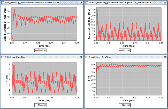
files. Several line plot examples are shown in Figure 13.6: Line plots created in Forte Monitor. The parameters plotted include mass flow rate at the Suction_Inlet
(open_boundary_flow.csv), torque on Left_Rotor
(rotation_boundary_parameters.csv), pressure monitored by monitor
probe P_high (P_high.csv), and temperature monitored by monitor probe
P_outlet (P_outlet.csv).
is a convenient tool for displaying these averaged solutions. Launch
Forte Monitor and open the .analysis directory of the Forte project to load the CSV
files. Several line plot examples are shown in Figure 13.6: Line plots created in Forte Monitor. The parameters plotted include mass flow rate at the Suction_Inlet
(open_boundary_flow.csv), torque on Left_Rotor
(rotation_boundary_parameters.csv), pressure monitored by monitor
probe P_high (P_high.csv), and temperature monitored by monitor probe
P_outlet (P_outlet.csv).
Ansys EnSight is the preferred tool for visualizing the spatially resolved solutions. Launch EnSight and open the .ftind file to load the solutions. The .ftind file is a solution index file, which contains the records pointing to a group of .ftres files. The actual solution data are contained in the .ftres files. If you need to control which .ftres solution(s) to load in EnSight, you can truncate or concatenate the records contained in the .ftind files in a text editor. Refer to the Forte User's Guide for details.
It is worth noting that the end gaps between the rotor end surfaces and the casing end surfaces are not meshed using fluid cells in the current setup. Although these end surfaces are part of the surface solutions, solution variables are not properly defined or extrapolated on them, therefore, they should not be used in visualizing the solutions in EnSight. These surfaces are highlighted in Figure 13.7: Post-processing the compressor simulation results using EnSight.
On the EnSight Part tree shown in Figure 13.7: Post-processing the compressor simulation results using EnSight, the last Part, VolumeCells, is the one that contains the 3D volume solutions. It can be used for creating clip-planes, iso-surfaces, particle traces, etc. Figure 13.8: Sample Forte simulation results visualized in EnSight shows several sample solution visualization images. In this example, the surfaces shown include all the bounding surfaces (excluding those highlighted in Figure 13.7: Post-processing the compressor simulation results using EnSight) and an XY-clip-plane (using VolumeCells as the parent) at Z = 0.05 cm.