Ansys Forte supports simulations of the following types of compressors:

Rotary-lobe compressors

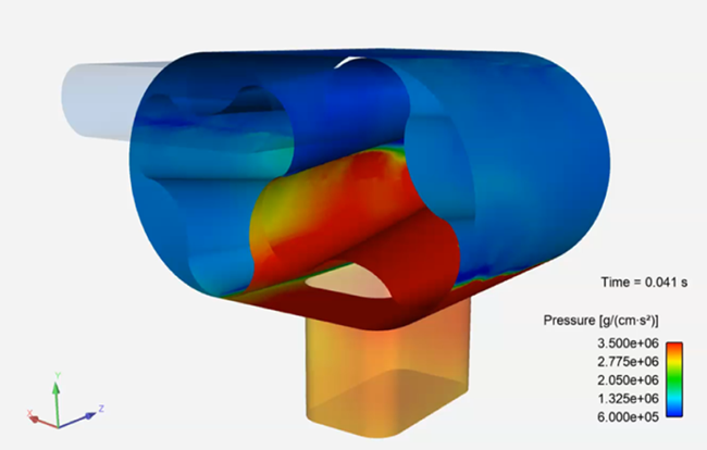
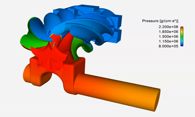
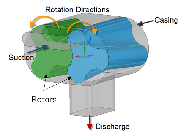
This type of compressors includes Roots blowers and screw compressors. Both use two intermeshing rotors, and the motion of each rotor is simple rotation. Roots blowers typically use cycloid rotors while screw compressors typically use helical rotors. Figure 5.1: Simulation of Roots Blower Compressor in Ansys Forte and Figure 5.2: Simulation of Screw Compressor in Ansys Forte show two examples. In the latter example, the compressor housing's casing surface is hidden to display the rotary screw lobes.

Figure 5.1: Simulation of Roots Blower Compressor in Ansys Forte

Figure 5.2: Simulation of Screw Compressor in Ansys Forte

Scroll Compressors

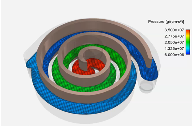
Scroll compressors use two interleaving scrolls of the same shape to compress the working fluids. One of the scrolls is static, and the other moves in an orbiting motion. Figure 5.3: Simulation of Scroll Compressor in Ansys Forte shows an example.

Figure 5.3: Simulation of Scroll Compressor in Ansys Forte

Reciprocating/Piston Compressors

The reciprocating or piston compressors use pistons driven by a crankshaft to compress gases. The methodology to set up such a simulation is similar to that used in setting up internal combustion engine simulations. Therefore, users may refer to the relevant content in Setting Up Generic Engine Cases with Valve Motion Using Automatic Mesh Generation. This section focuses on compressors with rotating motions, such as rotary-lobe and scroll compressors.

Piston Compression Pump With Built-in FSI in the Ansys Forte Tutorials provides an example of piston compressor, in which the piston moves with a slider crank motion to compress gas.

In compressor simulations, Ansys Forte uses its three-dimensional transient compressible flow solver to simulate the flow processes. The flow solver uses Arbitrary-Lagrangian-Eulerian (ALE) method to solve governing flow equations. It supports both Reynolds-Avearged-Navier-Stokes (RANS) and Large Eddy Simulation (LES) turbulence models. The transient time step sizes are adaptively adjusted for the benefits of efficiency and stability.

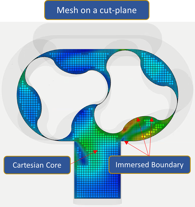
Ansys Forte uses Cartesian meshes generated by a parallel Octree-based solver with an immersed boundary method. The Cartesian meshes are generated automatically on the fly during the simulation. Load balance is dynamically adjusted in parallel computation. No meshing effort is required from the user prior to the simulation. See an example of the automatic meshing employed by the simulation in Figure 5.4: Octree-based Cartesian mesh in a compressor simulation.

Figure 5.4: Octree-based Cartesian mesh in a compressor simulation

Ansys Forte supports both ideal gas and real gas equations of state to model the working fluid. For refrigerant compressors, more discussion of the working fluid can be found in Refrigerant Properties.

The steps of setting up a simulation depend on the specific type of compressor. Refer to the content in Simulation of Rotary Lobe Compressors and Simulation of Scroll Compressors. Here, some general information is provided:

Import surface geometry

See Geometry Preparation and Fluid Volume Formation for general guidance.

Set up mesh refinement controls

These include surface refinements, Solution-Adaptive-Meshing (SAM) refinements, and gap feature refinements for small gaps. Handling of small gaps is critical in compressor simulations. See Small Gap Handling for more information.

Define boundary conditions and initial conditions

The motion of the rotating parts must be properly defined in boundary conditions. See Boundary Motion Specification for more information.

Set simulation controls and output controls

It is good practice to preview the simulation after it is set up. This is covered in Simulation Preview Through Ensight.

Surface Geometry Requirement

The surface geometry must be watertight. Specifically:

Figure 5.5: Surface Geometry in a Compressor Simulation

Preferred Preparation Approach

To generate watertight surface, it is recommended to use Ansys SpaceClaim and Creating "solids" for the simulation domain. After the geometry is prepared, export the surface mesh in .tgf (or .stl) format and import it into Ansys Forte.

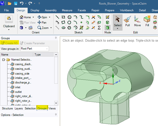
It is recommended that you take advantage of the Named Selection feature in Ansys SpaceClaim (Figure 5.6: Creating Named Selection (NS) in Ansys SpaceClaim). Named Selection allows you to denote different parts of the surface geometry separately. When importing the surface mesh into Forte, it uses the same naming convention for these parts. This helps specifying boundary conditions and mesh refinement controls in Forte. If you need to make adjustment to the geometry in SpaceClaim, the new surface mesh will replace the old one seamlessly in Forte if the naming convention remains the same.

Figure 5.6: Creating Named Selection (NS) in Ansys SpaceClaim

Fluid Volume Formation

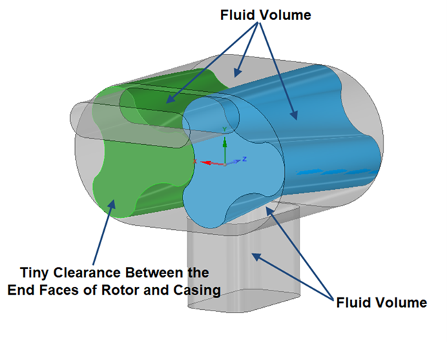
In a compressor simulation, fluid volumes are formed based on dynamically adjusted boundary positions. As shown in Figure 5.7: Fluid Volume Formation in a Compressor Simulation, the rotating rotor surfaces and the casing surface form several fluid volumes.

Figure 5.7: Fluid Volume Formation in a Compressor Simulation

Requirement on Material Point and Surface Normals

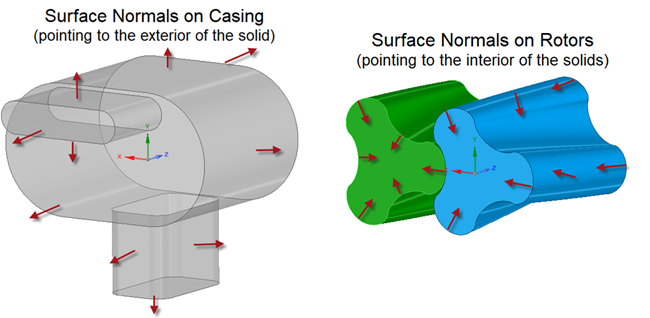
When setting up the simulation in Forte, the Material Point must always lie inside the fluid domain. Surface normals are required to point to the exterior of the fluid domain. As shown in Figure 5.8: The Directions of Surface Normals on the Casing and the Rotors, surface normals on the casing should point outwards, while those on the rotors should point inwards. In both cases, the directions of the normal are consistently pointing from the fluid domain to the solids.

Figure 5.8: The Directions of Surface Normals on the Casing and the Rotors

Rotational Motion Setup

To set up the motion of rotors in rotary-lobe compressors, one needs to define a Wall Boundary Condition. Select surfaces that form the rotating boundary, and select Rotation as the Motion Type. Then, define the rotation axis (origin and direction), and set the angular velocity. The sign of the angular velocity follows the right-hand rule regarding the rotation axis. These parameters are illustrated in Figure 5.9: Setting up Rotational Motion for a Rotor on the Wall Boundary Condition Panel.

Figure 5.9: Setting up Rotational Motion for a Rotor on the Wall Boundary Condition Panel

Orbiting Motion Setup

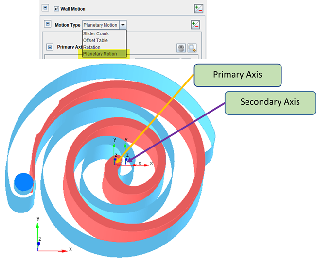
Typically, a scroll compressor has a static scroll and an orbiting scroll. While the static scroll is a stationary wall, the orbiting scroll should use Planetary Motion as Motion Type in its wall boundary condition setup.

To specify the planetary motion, you need to set up both the primary axis and the secondary axis of the rotation. The angular velocities of the primary and secondary rotations have the same magnitude but opposite signs. Figure 5.10: Setting up Planetary Motion for the Orbiting Scroll in a Scroll Compressor provides an example. The distance between the primary and secondary axes is the eccentric radius of the orbiting motion.

The location of the primary axis is fixed, while the location of the second axis specified in the UI corresponds to its initial position in the surface mesh (based on the orbiting scroll's initial position). During the orbiting motion, the secondary axis rotates around the primary axis at the primary rotation speed, and the orbiting scroll rotates around the secondary axis at the secondary rotation speed.

Figure 5.10: Setting up Planetary Motion for the Orbiting Scroll in a Scroll Compressor

Small gaps between the solid surfaces are common in compressor simulations, as they exist between the rotors and between the rotors and the casing. Flows through these gaps should be simulated since they are critical for how the compressor functions.

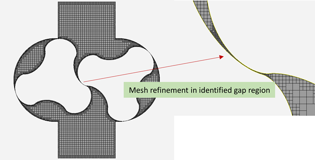
However, typical gap sizes are on the order of 50 μm. Resolving them would require micron-level cells and incur impractical computational cost. Ansys Forte does not rely on using micron-level tiny cells to resolve the gaps. When setting up Forte's simulation, the Cartesian cells in the gap region can be larger than the local gap size. Figure 5.11: Mesh Refinement in the Small Gaps in a Compressor Simulation shows how the typical local mesh resolution looks like. The mesh resolution in the gaps is refined relative to the global mesh size, but it remains coarser than the smallest gap spacing to control computational cost.

Figure 5.11: Mesh Refinement in the Small Gaps in a Compressor Simulation

Figure 5.12: Gap Feature Refinement Panel under Mesh Controls

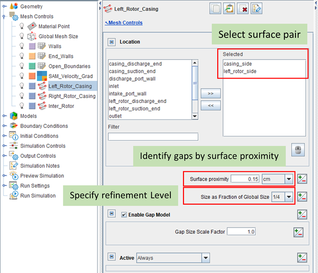
It is recommended to use Gap Feature Refinement (under Mesh Controls) to define the gap region and to apply mesh refinement to it. This feature is designed to detect small gaps between any two surfaces automatically. As shown in Figure 5.12: Gap Feature Refinement Panel under Mesh Controls, you first need to select a pair of surfaces that form the gap.

Gap region is automatically determined as where the spacing between the two surfaces is smaller than the "Surface Proximity", which is an empirical parameter. Starting from Ansys 2024 R2, surface proximity can be automatically determined by Forte. Select Determine from Surface Depth, which is the recommended default option. The Gap Feature Refinement applies mesh refinement to the identified gap region, based on the specified refinement level (Size as Fraction of Global Size).

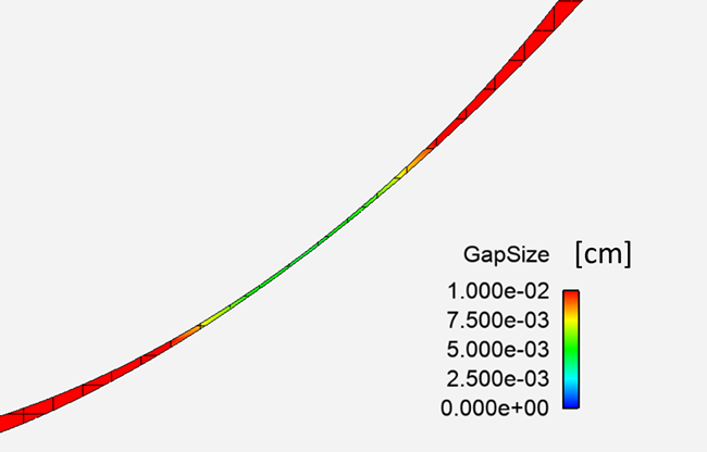
The spacing between the two surfaces (the local gap size), is measured accurately and dynamically during the simulation even as the two surfaces move. To check the local gap size in your simulation, you may open Forte's spatially-resolved solution in Ansys EnSight, apply a cut plane through the surfaces that form the gap, and color it with the "GapSize" variable, as shown in Figure 5.13: Checking Local Gap Size using the GapSize variable in Ansys EnSight. In this example, the smallest gap size between the two surfaces is around 50 μm.

Figure 5.13: Checking Local Gap Size using the GapSize variable in Ansys EnSight

To model the thermodynamic relations and properties of the working fluid, Ansys Forte supports both ideal gas and real gas model options. These options are accessed via Equation of State, shown in Figure 5.14: Selection of Equation of State on the Chemistry/Materials Panel . Specifically:

Figure 5.14: Selection of Equation of State on the Chemistry/Materials Panel

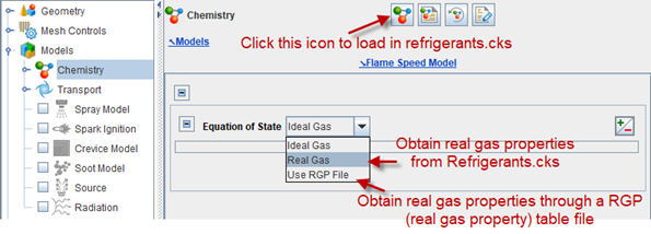
Ideal Gas: Ideal gas equation of state. This option is sufficient for compressors that use air as the working fluid.

Real gas: Real gas equation of state. This option is often necessary if the compressors use refrigerants as the working fluid. The real gas equation requires certain parameters that are specific for the fluids. These parameters are available from the chemistry sets provided by Ansys Forte's installation. For refrigerants, the chemistry set file Refrigerants.cks can be found in your Ansys installation:

\ANSYS Inc\v[release_number]\reaction\forte.win64\data

The following types of refrigerant fluids are included in the refrigerant library of Forte:

Use RGP File: use real gas properties are obtained through a RGP table file. This option requires a RGP file containing the tabulated thermodynamic data of the fluid to be simulated.

We recommend that you preview the simulation settings prior to starting the simulation. This is done on Preview Simulation > Mesh Generation, shown in Figure 5.15: Preview the Simulation with Mesh Generation.

Figure 5.15: Preview the Simulation with Mesh Generation

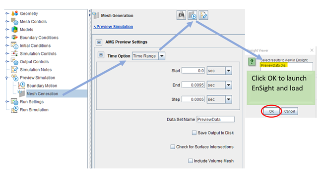
There are several options to generate the mesh in this simulation preview:

Option 1: Only check boundary motion. Do not select Check for Surface Intersections or Include Volume Mesh. In this case, preview solutions show up in EnSight almost instantly.

Option 2: Turn on Check for Surface Intersections. If there are any intersections between the surfaces, they are shown as part "Intersections" in EnSight. Slightly longer CPU time is expected using this option.

Option 3: Turn on Include Volume Mesh. This option checks the process of CFD mesh generation that would happen in the simulation. It is useful for checking Material Point position, surface normals, and mesh refinements. Longer CPU time is expected using this option. Try to use MPI mode and do limited number of snapshot checks only.

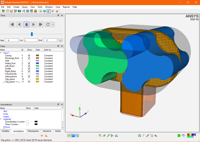
During the preview mesh generation, you can view the results in Ansys EnSight. Transient updates on the mesh are sent directly and dynamically to the EnSight instance. Figure 5.16: Compressor Simulation Preview in EnSight shows a cut plane through the simulation domain with CFD mesh displayed. The full suite of EnSight tools can be used to probe and visualize the mesh.

Figure 5.16: Compressor Simulation Preview in EnSight

Torque, power and axial force are the part of the spatially-averaged outputs introduced in Spatially Averaged and Spray Panel in the Ansys Forte User's Guide. They are activated in simulations with wall boundary's motion set as Rotation or Planetary Motion. In Table 5.1: Calculation of Torque, Power and Axial Force, the formulations used to compute these quantities are reviewed. Note that the torque's definitions are different between the two motion types.

In these formulations:

Table 5.1: Calculation of Torque, Power and Axial Force

	Rotation Boundary	Planetary Motion Boundary
Torque
Power
Axial Force

All the three quantities (torque, power, and axial force) are defined as being applied FROM the rotating/planetary-motion boundary ON the fluid. The sign conventions used in these output calculations are: