The following sections of this chapter are:
The following sections of this tutorial are:
- 1.1.1. Fluent Airflow on a Rough NACA0012 Airfoil
- 1.1.2. Droplet Impingement on the NACA0012
- 1.1.3. Fluent Icing Ice Accretion on the NACA0012
- 1.1.4. Postprocessing an Ice Accretion Solution Using CFD-Post Macros
- 1.1.5. Multi-Shot Ice Accretion with Automatic Remeshing
- 1.1.6. Multi-Shot Ice Accretion With Automatic Remeshing – Postprocessing Using CFD-Post
- 1.1.7. FENSAP Airflow on the Clean NACA0012 Airfoil
- 1.1.8. FENSAP Airflow Solution on the Rough NACA0012 Airfoil
- 1.1.9. Scheduling a Sequence of Runs With Fluent Icing
This tutorial is divided into the following sections:
The objective of this tutorial is to obtain an airflow solution around a rough NACA0012 airfoil, using Fluent Icing, that is suitable for icing calculations.
This tutorial demonstrates how to do the following:
Setup a rough Fluent airflow on an airfoil.
Compute the solution.
Examine the results.
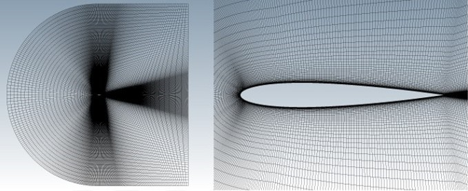
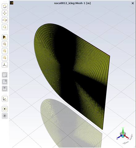
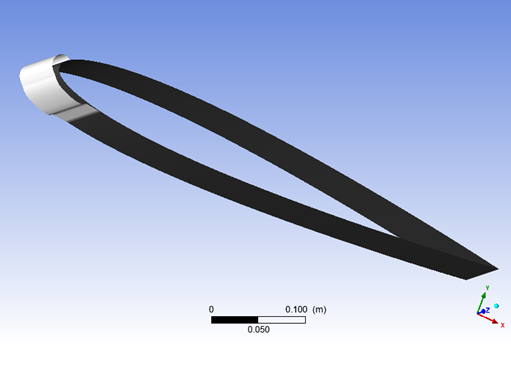
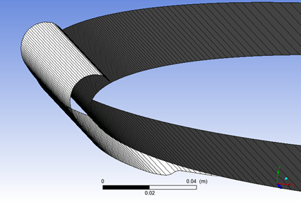
The problem considers the rough flow of air around a NACA0012 airfoil. Since the flow is viscous and turbulent, grid points have been clustered around the airfoil to better capture the boundary layer and wake.
The following sections describe the setup and solution steps for this tutorial:
To prepare for running this tutorial:
Download the
fluent_icing.zipfile here .Unzip
fluent_icing.zipto your working directory.The file, naca0012.cas.h5, can be found in the folder.
Use the Fluent Launcher to start Ansys Fluent.
In the Fluent Launcher, set the Capability Level to Enterprise, then select Icing.
Set Solver Processes between
2and4.Click Start.
Alternatively, Fluent Icing can be opened using the icing (on Linux) or icing.bat (on Windows) file inside the fluent/bin/ folder.
Uncheck , , and .
 Project
→ Workspaces →
Options
Project
→ Workspaces →
Options
The graphical user interface (GUI) of Fluent Icing is very similar to Fluent, however there are some differences such as:
The ribbon is reduced to only the File, Project, Results tabs and therefore most actions for setting up your simulation will be performed in the Outline View.
Individual settings are defined in the Properties window which is accessed by left-clicking an item in the Outline View.
Note: Settings in the Properties window are saved as you define them, unlike dialog boxes which require you to click an button.
The console allows for Python scripting, and can read Python commands from a journal / script file.
Create a new project file.
File → New
Project...
Enter
Fluent_Icing_NACA0012as the Project file name within the Select File dialog.Select and import the naca0012.cas.h5 input grid.
Project
→ Simulation → Import
Case
A New Simulation window will appear. Enter the Name of the New Simulation as
naca0012_icing, and check to enable . Click .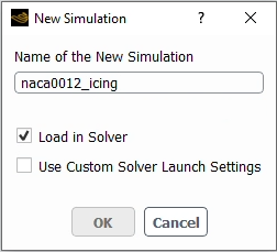
A dialog will open asking you to set the operating pressure to 0 Pa. Press to accept this change.
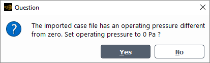
Note: Absolute pressure is recommended in all icing simulations. Therefore, Fluent Icing will automatically detect the imported case file, whose operating pressure is not equal to zero, when importing the case file. See Airflow in the Fluent Workspaces User's Guide for more details.
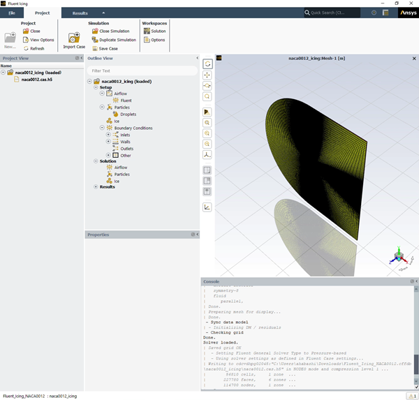
A new simulation folder will be created in the Project View, and the naca0012.cas.h5 file will be imported.
After the .cas.h5 file has been successfully loaded, a new Outline View tree appears under naca0012_icing (loaded).
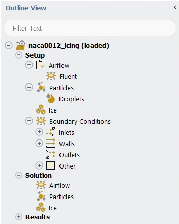
The mesh is now displayed in the Graphics window to the right.
Define the Simulation Type.
 Setup
Setup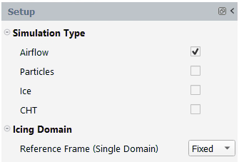
Enable and disable , and under Simulation Type within the Setup panel.
Set the Airflow properties for the simulation.
Setup → Airflow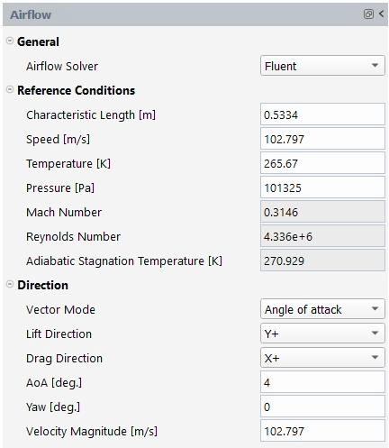
In the General section:
Retain the default selection of for Airflow Solver.
In the Reference Conditions section, retain the following settings:
0.5334for Characteristic Length [m].102.797for Speed [m/s].265.67for Temperature [K].101325for Pressure [Pa].
In the Direction section, retain the following settings:
for Vector Mode.
for Lift Direction.
for Drag Direction.
4for AoA [deg.].0for Yaw [deg.].102.797for Vector Magnitude [m/s].
Set the Fluent properties for the simulation.
Setup →
Airflow → Fluent
 Set to Default Air
Properties
Set to Default Air
PropertiesA dialog will open. Click to accept the air properties computed from the current airflow temperature.
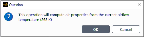
Note: This automatically sets the air properties, suggested for icing simulations, from the current reference air temperature. The values of air properties have been computed using the equations presented in Airflow.
For simplicity, thermal conductivity and viscosity equations are shown below.
where
 refers to the ambient air static temperature,
and
refers to the ambient air static temperature,
and  ,
,  and
and  are equal to 0.00216176
W/m/K3/2, 288 K and
17.9*10-6 Pa.s,
respectively.
are equal to 0.00216176
W/m/K3/2, 288 K and
17.9*10-6 Pa.s,
respectively.Airflow properties under the Materials section are now automatically updated with values computed from the Reference Conditions under
Setup → Airflow.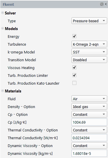
In the Solver section:
Retain the default selection of for Type.
In the Models section, retain the following settings:
Enable .
for Turbulence.
for k-omega Model.
for Transition Model.
Enable both Viscous Heating and Turb. Production Limiter.
In the Materials section, retain the following settings:
for Fluid.
for Density - Option.
for Cp - Option.
1004.69for Cp [J/kg-K].for Thermal Conductivity - Option.
0.0234394for Thermal Conductivity [W/m-K].for Dynamic Viscosity - Option.
1.68018e-5for Dynamic Viscosity [kg/m-s].
Open the Fluent Workspace.
Project
→ Workspaces → Solution
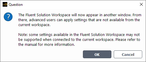
A dialog will open advising you that the Fluent Solution Workspace will appear in another window. Press to proceed.
Define the Viscous Model.
Setup →
Models → Viscous (SST
k-omega)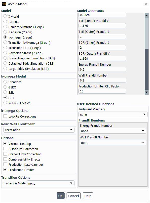
In the Model Constants section, retain the following settings:
0.9for Energy Prandtl Number.0.9for Wall Prandtl Number.
Press to close this window.
Define the Reference Values.
Setup →
Reference Values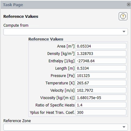
In the Reference Values section:
Retain all default values.
Define the Report Definitions.
Solution →
Report Definitions
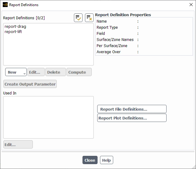
In the Report Definitions section:
Select report-drag and press (To create a new drag report, you can select → → )
Retain the default values of
0.99756405,0.069756474, and0for X, Y, and Z for Force Vector.Familiarize yourself with the selections in the Drag Report Definition dialog. Press to close this window.
De-select report-drag, select report-lift, and press (To create a new lift report, you can select → → )
Retain the default values of
-0.069756474,0.99756405, and0for X, Y, and Z for Force Vector.Familiarize yourself with the selections in the Lift Report Definition dialog. Press to close this window.
Press to close the Report Definitions dialog.
Modify the Absolute Criteria for convergence.
Solution → Monitors → Residual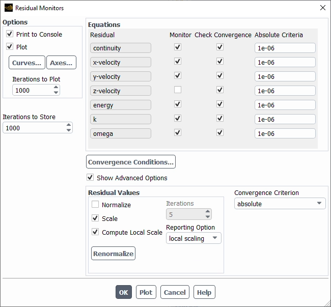
In the Equations section, retain the following settings:
1e-06for all Absolute Criteria entries.Enable and for all Residual fields.
Note: Since this 3D simulation provides a 2D solution, ensure to uncheck z-velocity under and keep enabled.
Enable .
Enable and .
Set Report Option to .
Press to close this window.
Maximize the Fluent Icing graphical user interface and close the Fluent Workspace.
Project
→ Workspaces → Solution
Set the Boundary Conditions for your simulation.
Setup → Boundary
Conditions → Inlets → pressure-far-field-4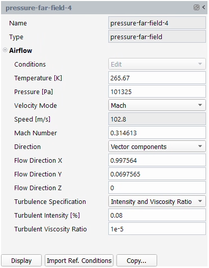
In the Airflow section:
Press to import the reference conditions of the case file.
Setup → Boundary
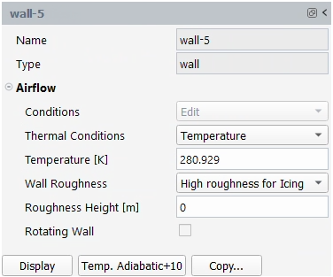
Conditions → Walls → wall-5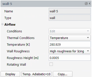
In the Airflow section:
Retain the default selection of for Thermal Conditions.
280.929for Temperature [K].Select under the Wall Roughness drop-down list.
Set Roughness Height [m] to
0.0005.Press on to ensure a temperature value (adiabatic temperature + 10 degree) is imposed on the wall.
Repeat the steps above for wall-6 and wall-7.
Note: To perform a simulation of a clean airflow solution:
Set Roughness Height [m] to
0.
Set the Solution properties of your simulation.
Solution → Airflow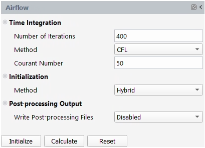
In the Time Integration section:
Set Number of Iterations to
400.Select under the Method drop-down list.
Retain the default value of
50for Courant Number.
In the Initialization section:
Select under the Method drop-down list.
In the Post-processing Output section:
Retain the default selection of for Write Post-processing Files.
Launch the simulation.
Solution → Airflow → A New run window will appear. Set the Name of the new run to
flow_rough.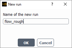
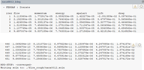
Once the computation is complete, the Airflow solution file, will be written inside the new run directory, naca0012_icing/flow_rough.
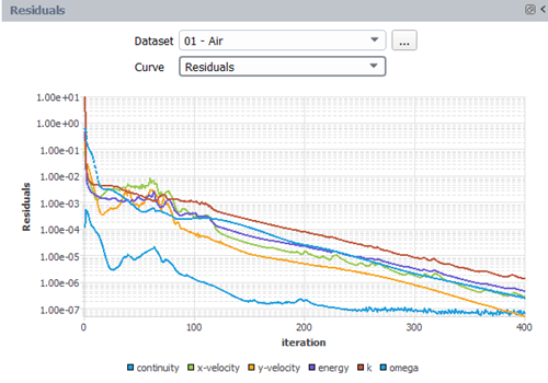
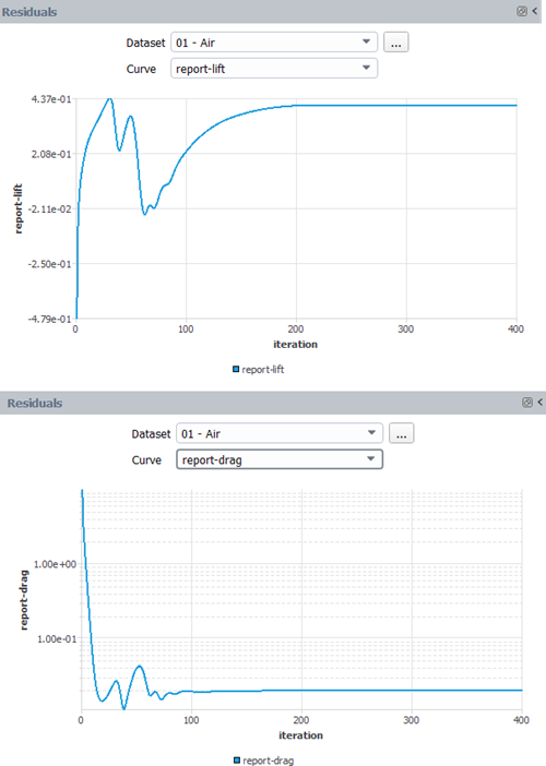
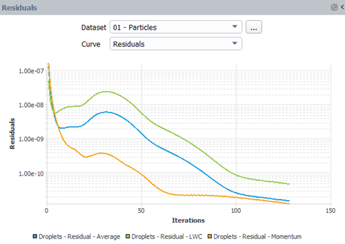
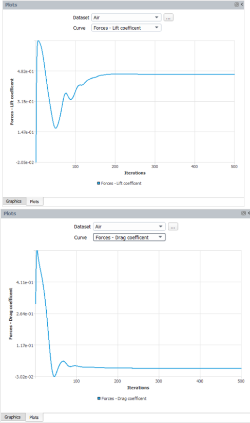
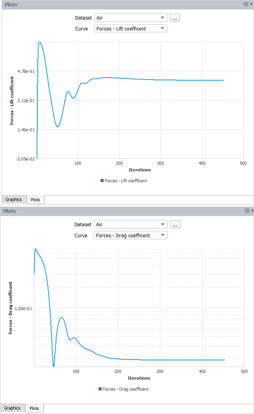
Take a look at the convergence history of this simulation in the Plots window located at the right of your screen. By default, the Plots window shows all Residuals of the governing equations at each iteration. It is possible to show the residual of a given governing equation by selecting the governing equation next to Curve located at the top of the Plots window. If other reports Reports have been defined in the original case file, they will appear as an option next to Curve. In this tutorial, the input case file contained lift and drag coefficient reports. Examine the convergence of these coefficients listed as report-lift and report-drag. Lift and drag coefficients have converged to 4.0570e-01 and 1.9850e-02 respectively.
The following three figures show the convergence of residuals and lift and drag coefficients.
Access the Quick-View options to better visualize the results of your simulation.
![]() Results
→ Quick-View
Results
→ Quick-View
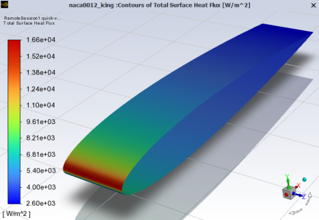
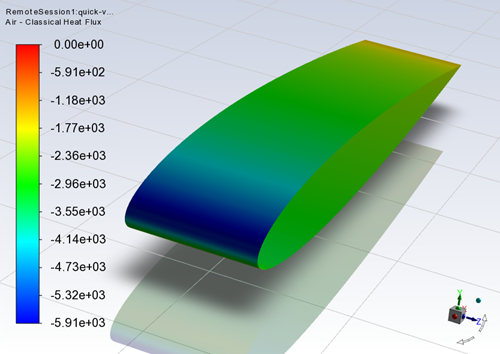
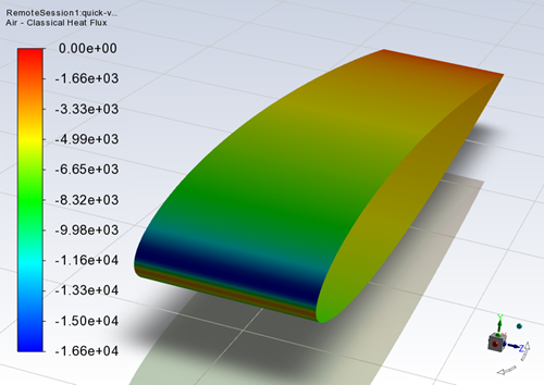
Visualize the convective heat flux over the NACA0012 airfoil.
Results
→ Quick-View →
Contour → A new quick-view-1 node is created in the Outline View which allows you to modify your heat flux properties.
Results → Contours → 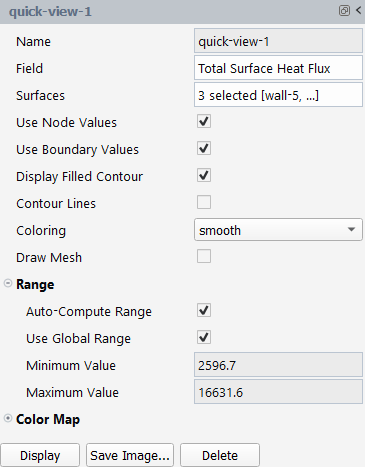
Modify your heat flux properties until you are satisfied with your view. Press to display the solution in the Graphics window. Press on to save your solution to an image file.
The objectives of this tutorial are to compute the droplet concentration around the NACA0012 airfoil and to compare the collection efficiency of a monodispersed droplet simulation to a statistically-distributed droplet diameter solution. Completion of Fluent Airflow on a Rough NACA0012 Airfoil is required before continuing.
In a monodispersed droplet calculation, a single droplet diameter represents the icing cloud that the aircraft is flying in. In reality, icing clouds never contain only one size of droplets but a distribution of droplet sizes. When running a single droplet diameter, the median volumetric diameter (MVD) of the droplets in the cloud is chosen as the monodispersed value. If a more accurate droplet solution is needed, then a distribution of droplet sizes can be solved for, where the MVD of this distribution matches that of the cloud.
You are invited to read Setting-up a Fluent Icing Simulation for more information on how to set up the input parameters of droplets and/or crystals.
Note: If you closed your Fluent Icing session since the completion of the last tutorial, you must reopen your project and load your previous simulation and settings. To do this, open Fluent Icing, select Project → , and navigate to and select your FLUENT_ICING_NACA0012.flprj project file. Once the project is opened, right-click the naca0012_icing simulation folder, and select . The simulation will be opened, and your window display will switch to the Outline View, with a simulation tree appearing under naca0012_icing (loaded). To ensure that you are working from the most recent settings, go back to the Project View, right-click the flow_rough run, and select . Particle simulation requires an airflow solution, therefore, to ensure that the solution of flow_rough is properly loaded into Fluent Icing, in Project View, right-click the out.dat.h5 file under flow_rough and select . Finally, go back to the Project tab to continue with the tutorial.
In this section, you will learn how to set-up and launch a monodispersed droplet simulation using Fluent Icing.
Select Project in the top ribbon and go to the Outline View. Select Setup under naca0012_icing (loaded). In its Properties window, make sure that Airflow and Particles are checked. Uncheck and .
Note: Setup, Solution and Results settings of the airflow around the NACA0012 have already been setup in In-Flight Icing Tutorial Using Fluent Icing. Therefore, they do not need to be updated.
Under Setup → Particles, activate Droplets in Type. Leave the other options unchecked.
Go to Droplets, inside Setup → Particles. In the properties window of Droplets,
Under Droplet Conditions, set the LWC [kg/m3] to
0.00055and the Droplet Diameter [microns] to20.Under Particles Distribution, keep Monodispersed since you will conduct a water catch simulation using a single droplet size.
Under Model, keep Water as the Droplet Drag Model. This is the default drag law for droplet particles.
Under Setup → Boundary Conditions, expand Inlets and go to pressure-far-field-4. In its properties window, under Particles, ensure is selected and remains unchecked. The option will apply the Droplet Conditions, located inside the Droplets window, at the inlet of the pressure-far-field-4, in this case, the LWC and the MVD. If remains unchecked, the airflow velocity is imposed as the droplet velocity at the inlet. The relative velocity between air and droplets is considered to be zero at far-field.
Note: When configuring particle flow simulations, boundary conditions are only specified at inlets.
Under Solution → Particles, set
300as the Number of Iterations under Run Settings. Keep the default settings in Solver and Initialization.Note: Inside Initialization, uses the airflow direction specified in Setup → Airflow as the initial velocity of droplets.
Right-click Particles under Solution and choose Calculate to launch the droplet particle simulation in standalone mode. A new window will appear requesting a name for the new run. Name the new run
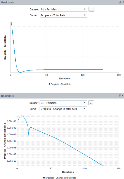
droplets_mvd.The calculation stops when the convergence level reaches the convergence limits set on the Residual cut-off and on the Change in total beta. Otherwise, the simulation continues until it reaches 300 iterations. In the Plots window, you can look at Residuals, Droplets – Residual – Average, Droplets – Residual – LWC, Droplets – Residual – Momentum, etc. curves and the Droplets -Total Beta and Droplets - Change in Total Beta convergence curves.
Often the solution in the wake of the droplet flow is still converging while the impingement at the surfaces is fully converged. If you wish to converge the wake and the shadow zones further, the Residual cut-off of the Particles panel under Solution should be reduced and the Number of Iterations should be increased. The droplet wake is usually not of interest and it is sufficient to achieve convergence of the total beta alone.
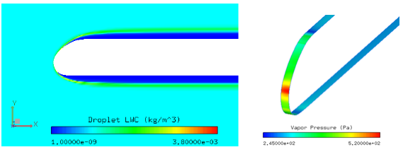
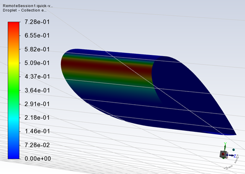
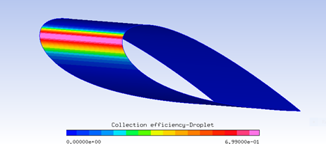
When calculations are completed, you may use Quick-View to view the results. Go to the ribbon bar of your Fluent Icing window and, under Results → Quick-View → , choose to output the water catch of the monodispersed droplets over the NACA0012. See Figure 1.10: Collection Efficiency of Monodispersed Droplets over a NACA0012.
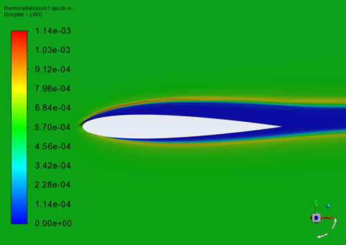
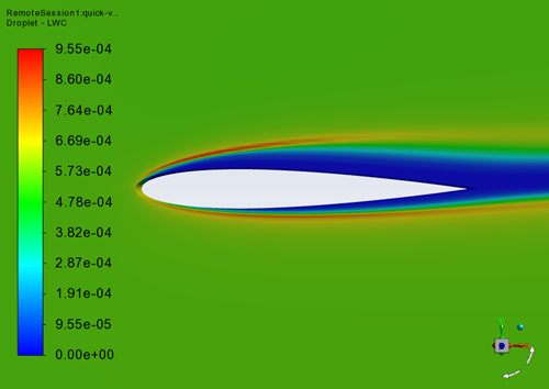
Repeat these steps to output the LWC around the NACA0012. Blue contours define the shadow zone where there is an absence of water droplets. See Figure 1.11: LWC of Monodispersed Droplets Around a NACA0012.
Select Project from the ribbon menu. Notice that naca0012_icing (loaded) simulation now contains the droplets_mvd run which contains the final Droplets solution. In addition to Quick-View, you can also open the results in Viewmerical from the . Right-click the Droplets solution and select → . A Viewmerical window will appear allowing you to further post-process the droplet results.
Note: The Droplets solution, shown in the Project View, is a link to a file on the disk. This link points to the filename naca0012.droplet. To show the filenames as they appear on the disk, you may right-click Name under Project View and select . Repeat these steps to disable before continuing with this tutorial.
Move on to the next tutorial, go back to the Project tab.
Caution: Do not close Fluent Icing.
There are several cloud droplet size distributions that have been published in the literature. The distributions published by Langmuir have been used by NACA to determine the MVDs currently listed in Appendix C, which is used for icing certification of aircraft. Advisory Circular No 20-37A from FAA suggests using Langmuir-D distribution for MVDs up to 50 microns. For more details on these distributions, you can consult the Advisory Circular, and also the book by Irving Langmuir, The Collected Works of Irving Langmuir (New York, Pergamon Press, 1960).
The most important reason for considering an analysis using a distribution is that there are droplets larger than the MVD in the distribution, which can impinge further back on the top and bottom of the airfoil, creating a thin but rough layer of ice that can have adverse effects on aerodynamics and control. In this case, solutions for each droplet size of a given distribution are calculated separately. The final solution is then created as a composite of all solutions using weights on each droplet size.
In this tutorial, you will use the set-up created in Monodispersed Calculation as a starting point.
Without closing the previous Fluent Icing session (Monodispersed Calculation), in the Outline View panel, go to Setup → Particles → Droplets. In the Droplets window, under Particles Distribution, set Droplet Distribution to .
Note: The current version of Fluent Icing supports pre-defined droplet size distributions (Langmuir B to E). User defined distributions are not yet supported. Below is a representation of a Langmuir D distribution and the droplet diameters that are used to represent this distribution.
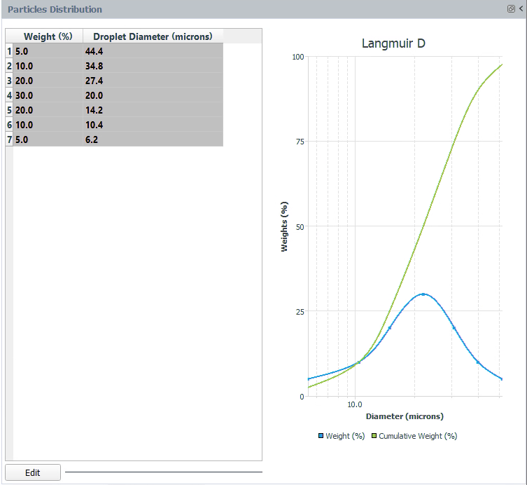
In the figure above, the droplet diameters are on the horizontal axis, and the weights (the percentage of droplets of a given diameter contained in the cloud) are on the vertical axis. The individual weights are shown with the blue curve, and the overall sum, cumulative weight, is shown with the red curve. On the red curve, the data points are plotted at the mid-range of their cumulative weight intervals. For example, the 20 microns droplet, which happens to be the MVD, covers the cumulative weight range of 35% to 65% and it is therefore plotted at 50% cumulative weight on the red curve.
A Particle droplet simulation is run for each droplet size shown in the above table.
Go to Solution → Particles. In its properties window, check Save Distribution Solutions under Output.
This will allow you to save a droplet solution for each droplet size simulated. Otherwise, only the combined solution of the distribution is saved. Keep all the other settings the same.
Right-click Particles under Solution, choose to run the calculation. A window will appear asking if you would like to continue the current run. Choose . A new run window will appear. Set the Name of the new run to
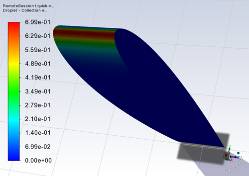
droplets_langd. Individual runs will be executed one after the other, and the results will be combined.When calculations are completed, you may use Quick-View to view the results. Go to the ribbon bar of your Fluent Icing window and, under Results → Quick-View → , choose to output the water catch of the Langmuir D droplet distribution over the NACA0012. See Figure 1.12: Collection Efficiency of Droplets with Langmuir-D Distribution over a NACA0012.
Repeat these steps to easily output the LWC around the NACA0012. Blue contours define the shadow zone, absence of water droplets. See Figure 1.13: LWC of Droplets with Langmuir-D Distribution Around a NACA0012.
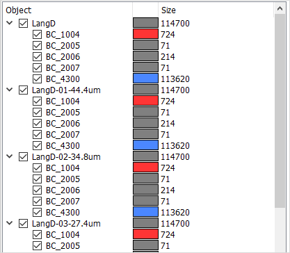
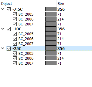
Select Project from the ribbon menu. Notice that naca0012_icing (loaded) simulation now contains the droplets_langd run. This run has a combined Droplets solution as well as each individual Droplets solution located in numbered folders d-01 to d-07.
To link each numbered droplet solution to a droplet size of the Langmuir D distribution, in the Project ribbon, select Project → → . A Project window appears. Click the + sign beside Metadata to expand the list of parameters associated to each run and solution. Scroll-down and select Droplets::D-Diam and click . A D-Diam column appears next to Name inside the Project panel. This column clearly identifies the droplet diameter used to obtain each solution.
Note: In addition to Quick-View, you may open the results in Viewmerical from the Project View. To display the combined droplet solution in Viewmerical, right-click the Droplets solution file and select → . Alternatively, to display an individual droplet solution file, right-click the d-0*/Droplets file of your choice and select → . A Viewmerical window will appear allowing you to further post-process the droplet results.
Before you move on to the next tutorial, go back to the Project panel.
Caution: Do not close Fluent Icing if you would like to proceed with the next section.
To complement the built-in post-processing, Ansys distributes Viewmerical and CFD-Post with the installation package. In this tutorial, you will use Viewmerical to post-process your droplet results. In the next tutorial, you will use CFD-Post to post-process your icing results.
Viewmerical is a light-weight graphical display tool specifically designed for in-flight icing solutions and applications. Viewmerical can display solution field contours, velocity vectors, planar cuts through the volumes, 2D graphs of variables, streamlines, etc. This tutorial will demonstrate some basic features of Viewmerical while comparing the two droplet solutions obtained in the previous sections.
In Project View, right-click the naca0012_icing → droplets_langd → Droplets solution and choose → . A message may appear asking if you would like to append this solution to a previously opened Viewmerical display. Click .
The program will launch and show an isometric display of the entire grid showing the first solution field, Droplet LWC, of the combined Langmuir D solution.
Rename this dataset by double-clicking the original name, data-naca0012.droplet. A Rename dataset window appears, write
LangDin the text box.Go to the Data tab and then change the Color range to .
Align the view angle with the Z-symmetry plane by right-clicking the 3D axes on the lower left, and by choosing . Alternatively, you can left-click the Z axis itself.
Zoom in on the airfoil. You can use Ctrl + left-click to draw a zoom box, or scroll the mouse wheel to zoom in and middle-click to pan.
Change the font of your legend to bold. Click
 on the top left corner of the window and select
Command window; then type
on the top left corner of the window and select
Command window; then type
BIGFONTSin the command line of the 3dview console and hit Enter. The legend fonts now become bold.Using the Camera icon on the upper left corner, you can take a snapshot of the solution window to capture the following image.
Figure 1.14: LWC of a Langmuir D Droplet Cloud over a NACA0012 at an AoA of 4 Degrees, Showing the Shadow Zone (Blue Region)
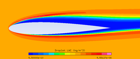
Examine the LWC distribution in the area close to the airfoil. The blue region is called the shadow zone, where no droplets exist. In between the shadow zone and the free stream, there are bands of high LWC concentrations which are the enrichment zones forming due to the constriction of stream tubes in the continuum domain. These features can be of special interest for downstream aircraft components.
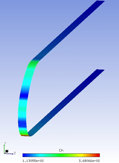
Go to the Data tab and choose Collection efficiency-Droplet. Collection efficiency is only displayed on the walls of your geometry. Go to the Objects tab and uncheck BC_1004 and BC_4300 to display the collection efficiency distribution only on the walls (BC_2005, BC_2006, BC_2007, and BC_2008).
Use the left mouse button to rotate, the middle mouse button to pan, and the right-mouse button to zoom in the airfoil surface to obtain the following figure.
Figure 1.15: Collection Efficiency of a Langmuir D Droplet Cloud on the Surface of the Airfoil at an AoA of 4 Degrees
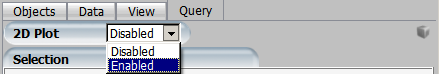
For a more in-depth quantitative view, it would be possible to create 2D data plots using Viewmerical. Click the Query tab and enable 2D Plot.
Change the Cutting plane to Z and the horizontal axis to Y.

On the lower right corner of Viewmerical, you can directly modify data sets and solution fields. Leave them as they are now.
The color and thickness of the data curve displayed in the graph can be changed by left-clicking the cube menu located on the top right and by choosing Curve Settings. Set the curve color to red and the curve widths to
2and press .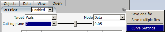
Finally, the following 2D plot is generated.
Figure 1.16: Collection Efficiency of a Langmuir D Droplet Cloud on the Surface of the Airfoil at an AoA of 4 Degrees
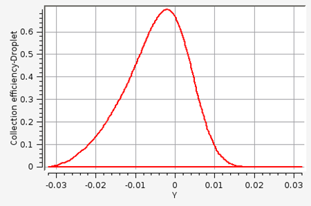
The maximum beta occurs at the stagnation point, just below the leading edge in this case. The points on the upper and lower surfaces where beta becomes zero are the impingement limits. In rime icing cases, all the water that impinges is frozen instantly, therefore icing limits are the same as the impingement limits. In glaze icing, water can runback and freeze past the impingement limits. Maximum beta is usually no more than 1.0, and reduces as the droplet flow becomes tangent to the surface.
To save data points of this collection efficiency distribution, go to the cube menu on the top right and choose . A new window pops up to browse and name the file that should contain these data points.
You can also open and compare several solution files using Viewmerical. Let’s display simultaneously all 7 droplet size solutions obtained in Langmuir-D Distribution.
Go to Project View. Under the run droplets_langd, right-click its d-01/Droplets file and select → .
A message appears asking if you would like to append this solution to a previously opened Viewmerical display. Click .
Inside Viewmerical, rename this new object by double-clicking its original name in the Object window and enter
LangD-01-44.4umin the window Rename dataset, where 01 indicates the droplet solution number and 44.4um is the droplet diameter of the droplet solution.Note: The droplet diameter of each droplet solution is shown in D-Diam column of the Project panel of the naca0012_icing (loading) simulation. See step 6 of Langmuir-D Distribution.
Repeat steps 14 to 16 to load the remaining droplet solutions from d-02/Droplets to d-07/Droplets.
Note: Alternatively, it is possible to bring each droplet solution by going to the run droplets_langd folder and by uploading each one of them from Viewmerical. To do this in Viewmerical, perform the following steps:
Click the
 button located at the right corner
of the Object panel. A window appears
to load a pair of files, a grid file and its solution
file.
button located at the right corner
of the Object panel. A window appears
to load a pair of files, a grid file and its solution
file.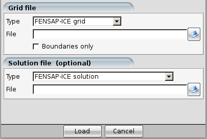
Click the
 folder icon of Grid
file and select the
naca0012.grid file located inside your
project and simulation directory
FLUENT_ICING_NACA0012/naca0012_icing/.
folder icon of Grid
file and select the
naca0012.grid file located inside your
project and simulation directory
FLUENT_ICING_NACA0012/naca0012_icing/.
Click the
folder icon of
Solution file (optional) and select the
naca0012.droplet.01 file located inside
your project, simulation and run directories
/FLUENT_ICING_NACA0012/naca0012_icing/droplets_langd.Press the button. A new data set is added to the Object panel. Rename this dataset by double-clicking its original name and enter
LangD-01-44.4umin the window Rename dataset, where 01 indicates the droplet solution number and 44.4um is the droplet diameter of the droplet solution.Repeat these steps for the remaining droplet solutions from naca0012.droplet.02 to naca0012.droplet.07.
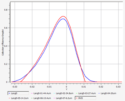
In Viewmerical, go to the Objects panel, uncheck LangD.
Go to the Data panel and click Shared located under Color range. Switch the Data field to Collection efficiency- Droplet.
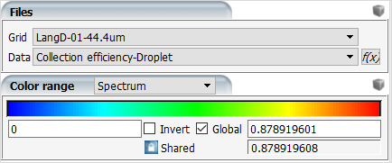
Go to the Query tab, enable 2D plot, and switch the Cutting plane to Z. The graph should display 8 individual beta distributions. Click LangD, to disable the LangD curve from the 2D plot. You can change the color and thickness of the data curve displayed in the graph via the cube menu on the top right and by choosing Curve Settings. You can also draw a zoom box by Shift + left-click.
Figure 1.17: Collection Efficiency on the Surface of the Airfoil at an AoA of 4 Degrees, Langmuir D Droplet Solutions
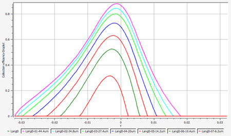
The curve with the lowest beta corresponds to the smallest droplet size (LangD-07-6.2 µm), and the one with the largest beta corresponds to the largest droplet size (LangD-01-44.4.µm). Smallest droplets are less ballistic, tend to follow the air flow and avoid the aircraft therefore reducing their collection efficiency and impingement limits. Larger droplets are more ballistic and they do not tend to follow the airflow. Therefore, their collection efficiency and impingement are usually higher than the smallest droplets. In general, this information is crucial to properly design the IPS power requirements and coverage.
Note: The difference between beta curves of different droplet sizes become more pronounced as the aircraft surface size increases. The effect can be dramatic on large blunt surfaces like fuselage noses or radomes where the contribution from the smaller size droplets can be negligible if compared to the largest ones. As a result, the composite or combined solution of a Langmuir simulation can be very different from the solution of the MVD.
To compare the LangD result to that of the monodispersed (MVD), go to the Objects panel, check LangD and uncheck all the other LangD-* objects.
Go to Project View. Under the run droplets_mvd, right-click its Droplets file and select → .
A message appears asking if you would like to append this solution to a previously opened Viewmerical display. Click .
Inside Viewmerical, rename this new object by double-clicking its original name in the Object window and enter
MVDin the window Rename dataset.Go to the Query tab, enable 2D plot, and switch the Cutting plane to . The graph should display 9 individual beta distributions. click LangD-01-44.4um to LangD-07-6.2um to disable these curves from the 2D plot. Change the color of the MVD to red and of the LangD to blue via the cube menu on the top right and by choosing Curve Settings. Set their width to
2. You can also draw a zoom box by Shift + left-click.The LangD solution is fairly close to that of the MVD. The impingement limits of the Langmuir D solution will always be further back due to the inclusion of larger droplets in the distribution. The maximum beta of the composite is lower than the MVD here. This is not always the case. Based on the size and shape of the impingement surface, the Langmuir D solution can have a maximum beta that is several times higher than the MVD. In this case, however, the results of the MVD and the distribution are close.
You will now compare the LWC of the largest and smallest droplet of a Langmuir D distribution. Go to the Objects panel, uncheck LangD and MVD objects and check LangD-01-44.4um (largest droplets) and LangD-07-6.2um (smallest droplets).
On the lower right corner of Viewmerical, change Collection efficiency-Droplet to Droplet LWC (kg/m^3).
Select LangD-01-44.4um in the Objects panel and choose Horizontal-Left under Split screen menu.
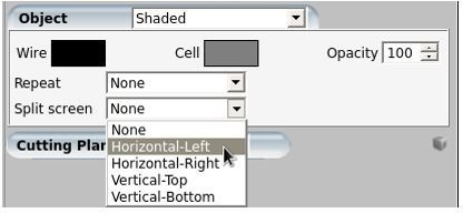
Go to the Data tab and change the color range to Spectrum 2 –16.
Align the view angle with the Z-symmetry plane and zoom in to capture the following image:
Figure 1.19: LWC Distribution and Shadow Zones for 44.4 Micron Droplets (Left) and 6.2 Micron Droplets (Right)
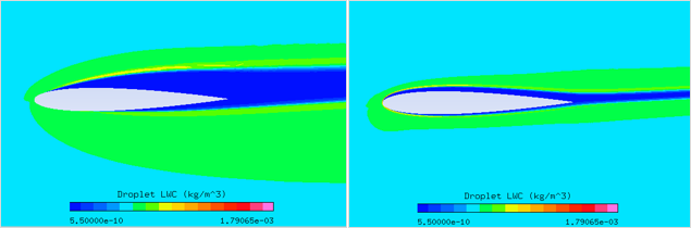
Observe the difference in the shadow zones. The smallest droplets follow the airfoil very closely but avoiding it while the largest droplets barely change their path and hit almost straight on, leaving a larger shadow zone.
The objective of this tutorial is to compute ice accretion and water runback on the NACA0012 airfoil at different icing temperatures. Icing temperature refers to the free stream air temperature at which the icing is to be computed. Inside Ice, this temperature can be different than what was used for the airflow free stream temperature. Indeed, the formulation of the heat fluxes in Ice allows you to use an air solution obtained at a temperature different than the intended icing temperature. In this manner, several icing temperatures can be investigated using the same airflow solution.
Note: The option to change icing air temperature in icing parameters is provided as a quick method to obtain different ice shapes with different ambient temperatures. It should be understood that this method is not identical in terms of accuracy to running air and droplet flows independently for each of those temperatures. Change in ambient air temperature would result in a proportional change in air density which would change the momentum transfer between air and particles. This would ultimately affect particle flow paths and collection efficiency. For internal flows, where particle thermal equation and/or vapor transport is enabled, icing air temperature should be kept the same as the reference air temperature.
You are invited to read Ice and Walls within the Fluent User's Guide for more information on how to set up the input parameters of the Ice module.
This tutorial will begin as a continuation of Monodispersed Calculation, so the monodispersed droplet solution and settings must be loaded.
Select Project from the top ribbon menu. To load the settings from the monodispersed run, right-click the droplets_mvd folder and select . To load the monodispersed solution, from the left side panel, right-click the droplets_mvd → Droplets solution file and select .
Note: If you closed your Fluent Icing session since the completion of the last tutorial, you must reopen your project and load your previous simulation and settings. To do this, open Fluent Icing, select Project → , and navigate to and select your FLUENT_ICING_NACA0012.flprj project file. Once the project is opened, right-click the naca0012_icing simulation folder, and select . The simulation will be opened, and your window display will switch to the Outline View, with a simulation tree appearing under naca0012_icing (loaded). Once this is done, continue with step 1.
Under Outline View, select Setup under naca0012_icing (loaded). In its Setup window, make sure that Airflow, Particles and Ice are checked.
Under Setup → Ice,
In Ice Accretion Conditions,
Check Specify Icing Air Temperature to simulate an icing temperature that is different than the reference/far-field air temperature.
Set the Icing Air Temperature [K] to
248.15K (-25 °C).
In Model,
Make sure that Icing Model is set to Glaze.
Leave the other settings as default.
In general, there is nothing to set in the Boundary Conditions of Ice unless icing is to be turned off on certain surfaces to reduce computational effort or sink boundaries are to be declared. Examine the options available for each wall without making any changes.
Go to Solution and change Log Verbosity to Complete to output extra execution and post-processed data in the Console window.
Go to the Solution → Ice,
Under Time, keep the Total Time of Ice Accretion [s] at 420 seconds and the option checked. The Ice feature in Fluent Icing is an explicit time-accurate code where the stability of the solution strongly depends on the value of the time step. The automatic time stepping option calculates the optimal stable time step at every iteration, which can change greatly depending on the size of the geometry and the mesh density.
Right-click Ice under Solution and choose to run the calculation. A window will appear. Name the new run
ice_mvd_m25C.After the simulation is complete, an Ice solution will be saved in the ice_mvd_m25C run folder.
Note: The Ice solution, shown in the Project View, inside the ice_mvd_m25c run, is a link to a file on the disk. This link points to the filename naca0012.swimsol. To show the filenames as they appear on disk, you may right-click Name under Project View and select . Repeat these steps to disable before continuing with this tutorial.
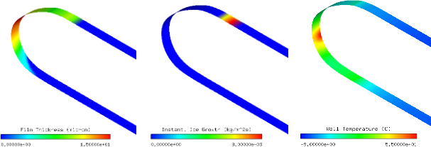
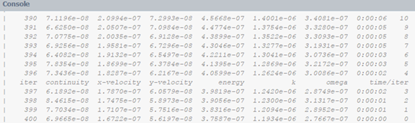
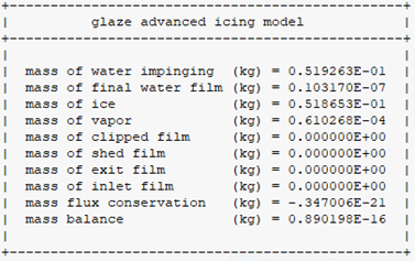
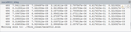
Look through the Console window of naca0012_icing. The accumulated time, value of the time step, total impingement, film, and mass of ice are printed at selected iterations. Heat flux and ice mass per wall boundary condition are listed in the following two tables. Finally, energy and mass conservation tables are printed. Most of the items in these tables are self-explanatory except perhaps mass of clipped film and runback flux. Clipped film refers to any film that is removed by sink boundaries and on certain nodes which collect and shed water (trailing edges, wing and blade tips, etc.) that are detected automatically. Runback flux is the sum of all edge fluxes in the domain which will be equal to the film removed by sink boundaries, or close to zero (mass conservation).
Cycle through the Plots window. By changing the Curve type, you will observe the progress of the total mass of ice, the change in instantaneous ice growth, water film thickness, and ice surface temperature with time. Since the input flow and droplet solutions are steady-state solutions, the icing solutions will eventually reach a steady-state where instantaneous ice growth, water film thickness, and ice surface temperature do not change after a while.
Go to the Ribbon menu and select Results. In Quick-View, click → to see the ice shape and the original surface in Viewmerical. If a window appears asking if you would like to append to a previously opened Viewmerical display, choose .
Alternatively, the ice cover solution can be loaded by going to the Project View, right-clicking Ice located in the ice_mvd_m25C run and selecting → . A window will appear, select as the view type. If a window appears asking if you would like to append to a previously opened Viewmerical display, choose .
You can change the option to other choices in the box to see the wireframe profiles and the surface meshes. In the panel, you can adjust the Ice thickness threshold based on ice growth to reduce display interlacing due to the overlapping of iced and clean surfaces.
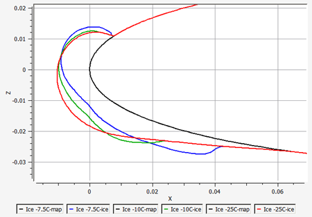
At -25 °C (248.15 K), the result is a pure rime ice shape.
Do not close the Fluent Icing session. You will now run two more calculations at warmer temperatures.
In the Outline View panel, select Setup → Ice and, in Ice Accretion Conditions, check Specify Icing Air Temperature and set the Icing Air Temperature [K] value to
263.15K (-10 °C).Right-click Ice under Solution and click to run the calculation. A window will appear. Name the new run
ice_mvd_m10C.Repeat steps 12 to 13 with an Icing Air Temperature [K] value of
265.67K (-7.48 °C). The same as the airflow Temperature [K] in Setup → Airflow → Conditions. Name this runice_mvd_m7p5C.Note: This -7.48 °C run is conducted at the same temperature as the airflow simulation. This is the standard usage of Fluent Icing, and most icing simulations will be run in this manner.
Since the icing air temperature is equivalent to the airflow simulation temperature, you can alternatively uncheck to disable it and Fluent Icing will use the airflow simulation temperature by default.
Now that there are three different ice shapes computed, you will analyze them using Quick-View. Go to the Ribbon menu and select Results. In Quick-View, click → . This opens the ice solution calculated in the previous simulation.
Rename this object by double-clicking its original name in the Object window and enter
Ice
                            -7.5C
in the window Rename dataset.To load the -10 °C and -25 °C solutions, go to Project View. Under the ice_mvd_m10C run, right-click Ice file and select → .
A message appears asking if you would like to append this solution to a previously opened Viewmerical display. Click .
A second message appears asking you to select the view type. In this case, select as you are going to compare the ice shapes produced by our simulations.
Inside Viewmerical, rename this new object by double-clicking its original name in the Object window and enter
Ice - 10Cin the window Rename dataset.Repeat steps 17 to 20 for the remaining ice shape, ice_mvd_m25C.
Click the button
 at the bottom
right of the data set list window located in the
Objects panel to enable all the grids in the 2D
plot.
at the bottom
right of the data set list window located in the
Objects panel to enable all the grids in the 2D
plot.Go to the Query panel and enable the 2D plot. Change the Cutting plane to and Mode to . At the bottom left of the 2D Plot window, set the horizontal axis to . Change the color and thickness of the curves by right-clicking the cube menu on the top right and then by choosing the menu.
Note: In this case, since all simulations were executed using a single ice accretion quasi-steady shot, each *-map curve represents the geometry of the NACA0012.
At -25 °C (248.15 K), the cooling effects are large, and all droplets freeze almost instantly producing a rime ice shape. This shape generally resembles the original airfoil profile and can be considered somewhat aerodynamic. As the icing temperature increases, more water can run back away from the stagnation zone and freeze where cooling effects become more predominant. This mechanism initiates the growth of ice horns on the upper and lower sides of the airfoil. These geometric features are common in glaze icing conditions and induce flow separation. Therefore they dramatically change the aerodynamic performance of the airfoil.
To properly capture the shape of the ice horns, a multishot computation is recommended where the grid, air and droplet solutions are updated at certain time intervals.
Finally, you will compare the film height of the three solutions. To do this, uncheck all Ice* objects located in the Objects panel of Viewmerical.
Go back to the Project View. Under the run ice_mvd_m7p5C, right-click its Ice file and select → .
A message appears asking if you would like to append this solution to a previously opened Viewmerical display. Click . A new Viewmerical window will be used to compare the solution values.
A second message appears asking you to select the view type. In this case, select as you are going to compare the solution fields of our ice simulations.
Inside Viewmerical, rename this new object by double-clicking its original name in the Object window and enter
-7.5C in the window Rename dataset.Repeat steps 25 to 28 for the remaining run folders, ice_mvd_m10C and ice_mvd_m25C. However, this time select to append these solutions to the previous solution.
In the Data panel, inside Files, choose Film Thickness as the Data field. Click Shared inside Color range.
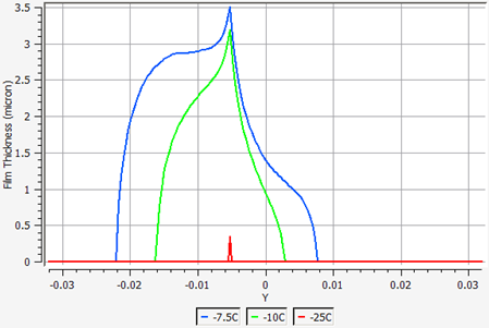
Go to the Query panel and activate the 2D plot. Set the Mode to Data and Cutting plane to Z. Set the horizontal axis to Y. The three curves showing the film height for the 3 different temperatures should be visible. Change the curve colors and thickness using the Curve Settings in the cube menu located at the top right.
The film height and extent grow with increasing icing temperatures. At -25 °C, almost all droplets freeze upon impact and there is no water runback on the surface. This temperature produces a rime ice shape. In the contrary, the amount of film and water runback of the other two cases clearly produce ice horns and form glaze ice shapes.
Caution: Do not close Fluent Icing if you would like to proceed to the next section.
In this tutorial, you will learn how to quickly post-process one-shot Ice results (ice shape and ice solution fields) using two dedicated CFD-Post macros: Ice Cover – 3D-View and Ice Cover – 2D-Plot. For this purpose, the icing solution of your icing simulation at -7.5 °C of Fluent Icing Ice Accretion on the NACA0012 is used and, therefore, completion of Fluent Icing Ice Accretion on the NACA0012 is required.
For more information regarding these macros, consult CFD-Post Macros within the FENSAP-ICE User Manual.
Note: CFD-Post only supports .h5 format files when beta features are enabled. Therefore, in order to ensure full compatibility with CFD-Post, first load CFD-Post, go to → . Inside the Options window, go to CFD-Post → General → Beta Options and check .
Inside your Fluent Icing window, go to the Ribbon menu and select Results. In Quick-View, click → .
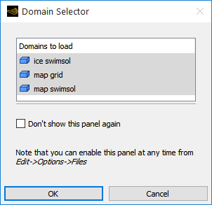
After opening CFD-Post, a Domain Selector window will request confirmation to load the following domains: ice swimsol, map grid, and map swimsol. Click to proceed.
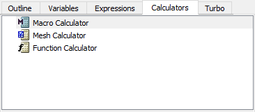
Go to the Calculators tab and double-click Macro Calculator. The Macro Calculator’s interface panel will be activated and displayed.
Note: The Macro Calculator can also be accessed by selecting Tools → Macro Calculator from CFD-Post’s main menu.
Select the Ice Cover – 3D-View macro script from the Macro drop-down list. This will bring up the user interface which contains all input parameters required to view ICE3D output solutions in the CFD-Post 3D Viewer.
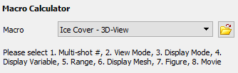
The default settings inside the Macro Calculator panel will allow you to automatically output the ice shape of a one-shot icing simulation by pressing Calculate. Figure 1.25: Ice View with CFD-Post, Ice Cover shows the output of the default settings of the macro.
Note: To change the style of the ice shape display, go to the Display Mode and select one of following options: Ice Cover, Ice Cover – shaded, Ice Cover – No Orig, Ice Cover (only) or Ice Cover (only) - shaded. To output the surface mesh of the ice shape, go to the Display Mesh and select Yes. Figure 1.26: Ice View in CFD-Post, Ice Cover with Display Mesh shows the output of activating Ice Cover under Display Mode by selecting Yes under Display Mesh and pressing at the bottom of the Macro Calculator.
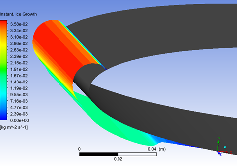
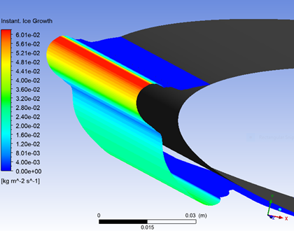
To display the solution fields of your icing simulation, you can either select Ice Solution – Overlay, Ice Solution or Surface Solution under Display Mode. In this case, you will output the ice accretion rate over the ice layer. To do this, select Ice Solution – Overlay in Display Mode, Instant. Ice Growth (kg s^-1 m^-2) in Display Variable and No in Display Mesh to turn off the displaying surface mesh.
Click Calculate to view the instantaneous ice growth over the ice shape. Figure 1.27: Ice View in CFD-Post, Instantaneous Ice Growth over Ice Cover Surface shows the output of the macro.
Note: You are invited to modify the input parameter of Display Variable to view different fields of the ICE3D solution.
You will now explore some quick post-processing capabilities of the Ice Cover – 2D-Plot macro. In the Macro drop-down list of the Macro Calculator panel, change the macro to Ice Cover – 2D-Plot.
Note: This switches the macro from Ice Cover – 3D-View to Ice Cover – 2D-Plot. Switch back to Ice Cover – 3D-View in the same way if needed.
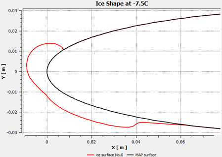
Change Plot’s Title from default, ICE SHAPE PLOT, to
Ice Shape at -7.5
                        C
, since you are creating a 2D-plot of the ice shape.Inside 2D-Plot (with),
Set Mode to Geometry to output an ice shape. The other options output the ice solution fields.
Set Cutting Plane By to Z Plane. Specify a Z=0 plane by setting X/Y/Z Plane to
0.Set the X-Axis to X and the Y-Axis to Y.
To center the 2D-Plot around the leading edge of the NACA0012, in 2D-Plot (with),
Change the (x)Range of the X-Axis from Global to User Specified. Specify values of
0.075and-0.01in the input boxes of (Usr.Specif.x)Max and (Usr.Specif.x)Min, respectively.Change the (y)Range of the Y-Axis from Global to User Specified. Specify values of
0.03and-0.03in the input boxes of (Usr.Specif.y)Max and (Usr.Specif.y)Min, respectively.
Leave the other default settings unchanged and click Calculate to create a 2D-Plot of the ice shape in ChartViewer. Adjust the output window’s size. Figure 1.28: 2D-Plot in CFD-Post, Clean Wall Surface and Ice Cover Surface shows the output of the macro.
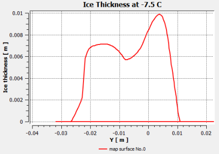
To create a 2D-plot of an ice solution field, first change the name of the plot. In this case, enter
Ice Thickness at -7.5 Cin the Plot’s Title field since you will create a water film 2D plot along the thickness of the airfoil.Inside 2D-Plot (with),
Set Mode to Solution (on Map Surfaces) to output the water film over the NACA0012. Selecting Solution (on Ice Surfaces) will output the ice field over the ice shape.
Set Cutting Plane By to Z Plane. Specify a Z=0 plane by setting X/Y/Z Plane to
0.Set the X-Axis to Y.
Set the Y-Axis to Ice Thickness (m).
To center the 2D-Plot around a meaningful scale to clearly see the water film distribution, in 2D-Plot (with),
Make sure that (x)Range of the X-Axis is set to User Specified. Enter values of
0.02and-0.04for (Usr.Specif.x)Max and (Usr.Specif.x)Min, respectively.Set (y)Range of the Y-Axis to Global. The macro will use the max./min. values of the water film thickness to define the range of the Y-Axis.
Leave the other default settings unchanged and click Calculate to update the 2D plot in ChartViewer. Figure 1.29: 2D-Plot in CFD-Post, Ice Thickness Distribution shows the output of the macro.
Note: You are invited to modify the input parameter of 2D-Plot (with) → Y-Axis to view different fields of the ICE3D solution.
As ice grows, the geometric profile of the contaminated airfoil changes which modifies the flow of air and water droplets around it. The quasi-steady multishot approach allows simulation of realistic and accurate ice shapes. In this approach, the total time of ice accretion is divided into smaller steady-state intervals (shots), where the mesh used to calculate the airflow, the droplet impingement, and the ice accretion is updated at the end of each shot to account for the ice shape. In this tutorial, you will use automatic remeshing with Fluent Meshing to rebuild a computational domain around the ice shape generated at each shot.
Note: Two approaches are supported in Fluent Icing to represent the computational domain at each shot: the automatic mesh displacement approach and the automatic remeshing with Fluent Meshing method.
The automatic mesh displacement uses the initial surface mesh to represent the ice shape. Surface nodes are moved inside the computational domain to represent the ice that forms at each shot. This process keeps the number of nodes and cells constant. As the ice shape grows, the total area covered by the boundary wall mesh increases which changes the size and the aspect ratio of the cells near the ice. This may result in a less than optimal grid spacing if the initial mesh is not fine enough. For complex ice shapes, manual remeshing maybe required in order to continue the multishot process when using automatic mesh displacement.
Alternatively, it is possible to use automatic remeshing with Fluent Meshing when simulating multi-shot icing. Remeshing refines and reorganizes the mesh topology on and around the ice. This leads to more stable and accurate air and droplet solutions for the next shot. Negative volume elements that often form with large mesh deformations are avoided with remeshing. For more information regarding automatic remeshing, consult Ice.
This tutorial is a continuation of the previous tutorial. The last run that was computed was the ice_mvd_m7p5C run. The current settings setup in the simulation panel will be consistent with the settings from that run. However, to be certain that you begin from those conditions, you may right-click the ice_mvd_m7p5C run in the Project View panel and select .
In the Outline View, go to Setup → Ice. In its Properties window, check Beading under Model. Beading is the roughness model of the Ice component. At the end of each shot, Beading will produce a roughness distribution that is used by the airflow solver (Fluent or FENSAP) during the next shot. This approach removes any arbitrary specification of roughness value. The first shot always needs some initial roughness, 0.5 mm in In-Flight Icing Tutorial Using Fluent Icing, since Ice is not run a priori. However, the remaining shots will use the distribution obtained from the beading model.
Note: Alternatively, the initial shots could be conducted over small time intervals where the surface roughness can be allowed to grow from 0 to a reasonable level, removing the need to specify an initial roughness value. For internal flows, you should start with a zero initial roughness instead. Roughness should be allowed to build progressively using shorter icing shots.
Click Solution and, in its Properties window, under Multi-shot:
Set Number of Shots to
3.Check Save Files at Each Shot to examine the steady-state solutions at the end of each shot.
At the start of each shot, the airflow can be initialized using the parameters defined in the case file () or the interpolated airflow solution from the previous shot (). This can be defined inside the Airflow Restart option. In the current simulation, leave it to , which is the default option.
Under Solution → Ice,
In Time, change the Total Time of Ice Accretion [s] from
420to140which corresponds to 1/3rd of the total time.Click , located at the bottom of the Ice panel. This automatically sets Fluent Meshing as the remeshing solver, and adds extra options, under Remeshing, to control the type of mesh refinement at each shot.
Below Remeshing, several options are available to control the surface mesh refinement as well as hexas (boundary layer cells) and prisms that will compose the computational domain at each shot. Enter the following settings as shown in the image below.
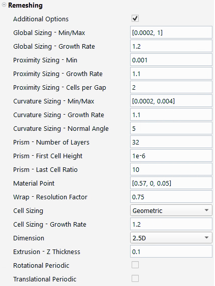
By selecting under Dimension, you are indicating to Fluent Meshing to generate a 2.5D mesh by extruding a surface mesh from one symmetry plane to the other. Therefore, there are some requirements that the initial case file that is imported into Fluent Icing must have:
Symmetry planes that represent the span of the airfoil must be Z planes. One of the two symmetry planes must be located at Z=0 and the other should be placed at a Z+ location.
Both symmetry planes must share the same zone name and type.
The material point must be located near the trailing edge and at half-span.
Below are some useful recommendations to consider based on the type of trailing edge that your 2.5D airfoil has:
Sharp trailing edge
Split the pressure and suction sides into two separated zone BCs. The trailing edge will be a geometric edge that separates these two BCs.
Blunt trailing edge
Put the blunt trailing edge surface in a separate zone BC.
For more information, consult Ice.
Right-click Solution and then select to automatically remove previous airflow, particles and ice solutions from memory.
Launch the multishot calculation by right-clicking Solution and then by selecting . A Warning message will appear highlighting the need to switch to in order to proceed with this multishot simulation. Select since the icing temperature must be identical to the airflow reference temperature when running a multishot simulation.
Another window will appear. Name the new run
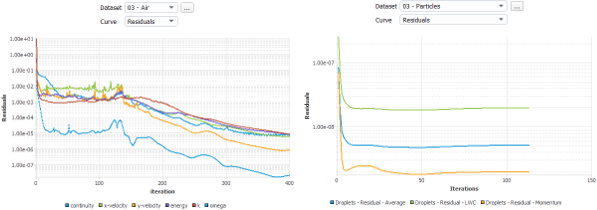
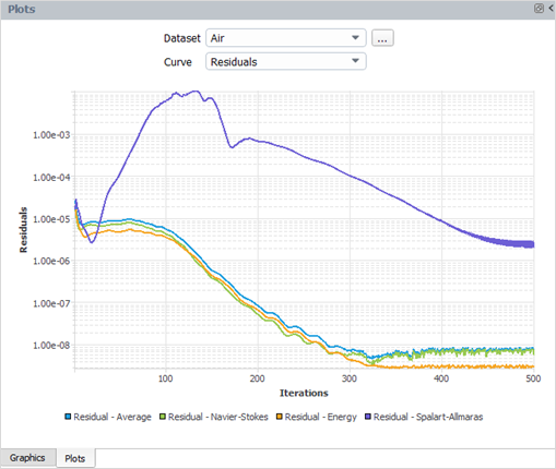
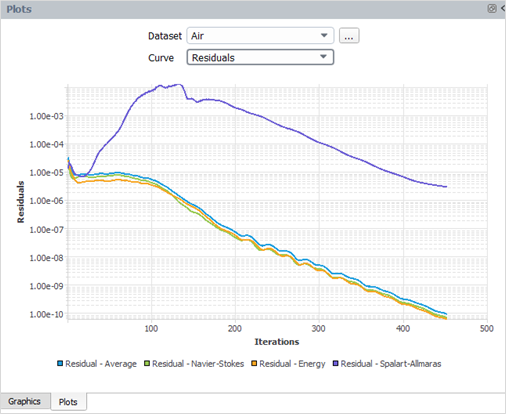
ice_mvd_m7p5C_multiand press .Go to the Plots window and monitor the convergence of Airflow, Particles and Ice solvers. In the Plots window, first select a shot and a solver next to Dataset, and then choose the residual or report to output next to Curve. The image below shows the residuals of the 3rd shot of the Airflow and Particles solvers.
Go to the Project View by clicking the Project tab in the top ribbon menu. Under the naca0012_icing (loaded) simulation, a new run named ice_mvd_m7p5C_multi now appears and is specified as (current). Expand the run by clicking the + icon to the left of ice_mvd_m7p5C_multi to show the files associated with the run. A shot.** folder is created for each shot of the icing calculation, and includes a two-digit number that links these folders to their shot number. Once all calculations are complete, view the final ice shape by following these steps:
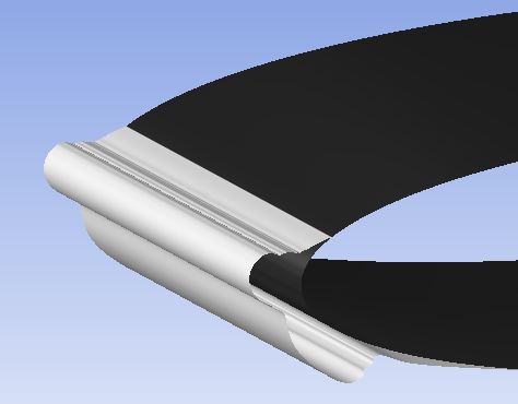
Right-click shot.01/Ice and select → to load the clean airfoil surface. Select if asked to append this solution to an existing Viewmerical window.
Right-clicking shot.03/Ice and select → to load the result of computed ice shape. Click when a message appears asking if you would like to append this to a previously opened Viewmerical display. A View Ice dialog will then open asking you to select the view type, select to proceed.
In Viewmerical, click the loaded clean airfoil surface grid-naca0012.01.map.grid under the Objects panel. In Object, select and double-click Cell to open the Select Color window. In this window, set the HTML color to #
474747and press .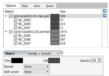
Click the loaded ice shape ice-naca0012.03.swimsol under the Objects panel. Make sure that is selected in Object. Go to the Data panel and select under the Display mode of ICE3D. Set the value to
0.1kg/m^2 under Ice thickness threshold.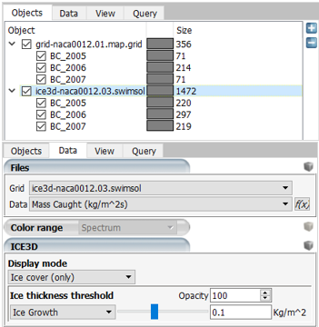
Go to the View panel. Set the Ambient light boost to a value of
20% under Global display settings.
After viewing this ice shape, close Viewmerical.
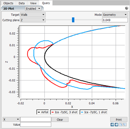
Next, compare the ice shape of the multishot run to that of the single shot run. Go to the Project View. Under the run ice_mvd_m7p5C_multi, right-click shot.01/Ice and select → . This grid file represents the surface grid (called naca0012.01.map.grid on disk) used to calculate the 1st shot of ice accretion.
Rename this object by double-clicking the grid-naca0012.01.map.grid object name and enter
Airfoilinto the Rename dataset window.Under the run ice_mvd_m7p5C_multi, right-click shot.03/Ice and select → . This grid file represents the ice surface grid (naca0012..03.ice.grid on disk) calculated during the 3rd shot of ice accretion.
A message appears asking if you would like to append this to a previously opened Viewmerical display. Choose .
Rename this object by double-clicking the grid-naca0012.03.ice.grid object name and enter
Ice -7p5C, 3 shots in the Rename dataset window.Under the run ice_mvd_m7p5C, right-click Ice and select → . This grid file represents the ice surface grid calculated during the single shot run.
A message appears asking if you would like to append this to a previously opened Viewmerical display. Choose .
Rename this object by double-clicking the grid-naca0012.ice.grid object name and enter
Ice -7p5C, 1 shotin the Rename dataset window.Click the Lock icon
at the lower
right of the data set list in the Objects
window.Go to the Query panel and activate the 2D plot. Set the Mode to and Cutting plane to . Set the horizontal axis to . The three curves showing NACA0012 and the ice shapes should be visible. Change the curve colors and thickness using the Curve Settings in the cube menu located at the top right. You can also draw a zoom box by Shift + left-click.
Note: The multishot simulation produces an upper horn that is more pronounced. This is mainly due to the continuous increase in collection efficiency and convective heat fluxes (cooling effects) as the upper horn curvature increases. The lower part of the ice is also thicker where the roughness has grown beyond the initial 0.5mm to about 1mm (average), which causes the water film to freeze sooner and show less runback compared to the single shot solution.
In this tutorial, you will learn how to quickly post-process and generate figures and animations of a multishot ice accretion simulation (ice shape and ice solution fields) using two dedicated CFD-Post macros: Ice Cover – 3D-View and Ice Cover – 2D-Plot. For this purpose, the multishot icing solution of Multi-Shot Ice Accretion with Automatic Remeshing is used and, therefore, completion of Multi-Shot Ice Accretion with Automatic Remeshing is required.
For more information regarding these macros, consult CFD-Post Macros within the FENSAP-ICE User Manual.
Inside your Fluent Icing window, go to the Ribbon menu and select Results. In Quick-View, click Ice Cover → Multi-shot Ice Cover – CFD-Post.
After opening CFD-Post, a Domain Selector window will request confirmation to load the following domains: ice swimsol, map grid, and map swimsol. Click to proceed.
Go to the Calculators tab and double-click Macro Calculator. The Macro Calculator’s interface panel will be activated and displayed.
Note: The Macro Calculator can also be accessed by selecting Tools → Macro Calculator from the CFD-Post’s main menu.
Select the Ice Cover – 3D-View macro script from the Macro drop-down list. This will bring up the user interface which contains all input parameters required to view ICE3D output solutions in the CFD-Post 3D Viewer.
The default settings inside the Macro Calculator panel will allow you to automatically output the ice shape for the first shot of the multishot simulation. Output the ice shape at the end of the multishot simulation of Multi-Shot Ice Accretion with Automatic Remeshing. This corresponds to the ice shape of shot 3, by specifying
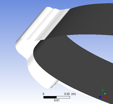
3for Multi-shot # and clicking Calculate. Figure 1.32: Ice View in CFD-Post, Final Ice Shape shows the output of the final ice shape.Note: To change the style of the ice shape display, go to Display Mode and select one of following options: Ice Cover, Ice Cover – Shaded, Ice Cover – No Orig, Ice Cover (only) or Ice Cover (only) - shaded. To output the surface mesh of the ice shape, go to the Display Mesh and select .
To display the solution fields of your icing simulation, you can either select Ice Solution – Overlay, Ice Solution or Surface Solution under Display Mode. In this case, you will output the ice accretion rate over the ice layer of the 3rd shot. To do this, select Ice Solution – Overlay in Display Mode, Instant. Ice Growth (kg s^-1 m^-2) in Display Variable and No in Display Mesh to turn off the displaying surface mesh.
Click Calculate to view the instantaneous ice growth over the ice shape. Figure 1.33: Ice View in CFD-Post, Instantaneous Ice Growth over Ice Cover Surface, Final Ice Shape shows the output of the macro.
You can also generate and save animations that highlight the ice shape evolution of your multishot simulation. Follow these steps to create and save a custom animation.
Set Multi-shot # to
1. The animation starts at the assigned shot number in Multi-shot # to the last shot of the simulation.Set (Multi-shot) Movie to On and click Calculate to see the animation on the 3D Viewer window.
To save this animation, in (Multi-shot) Movie,
Set Save to Yes.
Select an export Format. Two formats are supported, wmv and MPEG4. The default is wmv.
Specify a Filename.
Click Calculate to generate and save the animation. A message will appear to notify you of the location where the animation is saved and of the first shot used to generate the animation.
Note: If CFD-Post was opened using Fluent Icing, the animation will be saved in your run directory. If CFD-Post was opened in standalone mode, the animation will be saved in the Window’s system default folder.
Select Ice Cover – 2D-Plot from the Macro drop-down list to create 2D-plots of the multishot simulation. You will create a 2D-Plot that contains all the ice shapes generated by the multishot simulation.
Make sure that Multi-shot # is set to
1.Change Plot’s Title from ICE SHAPE PLOT, to
Multishot Ice Shape at -7.5 C (3 shots).Select Multi-Shots in 2D-Plot (with). The macro will generate a series of 2D plot curves, starting from the assigned shot number in Multi-shot # to the last shot of the simulation.
Inside 2D-Plot (with),
Set Mode to Geometry to output an ice shape. The other options output the ice solution fields.
Set Cutting Plane By to Z Plane. Specify a Z=0 plane by setting X/Y/Z Plane to
0.Set the X-Axis to X and the Y-Axis to Y.
To center the 2D-Plot around the leading edge of the NACA0012, in 2D-Plot (with),
Change the (x)Range of the X-Axis from Global to User Specified. Specify values of
0.06and-0.025in the input boxes of (Usr.Specif.x)Max and (Usr.Specif.x)Min, respectively.Change the (y)Range of the Y-Axis from Global to User Specified. Specify values of
0.025and-0.035in the input boxes of (Usr.Specif.y)Max and (Usr.Specif.y)Min, respectively.
Leave the other default settings unchanged and click Calculate to create a 2D-Plot of the multiple ice shapes in ChartViewer of CFD-Post. Adjust the output window’s size. Figure 1.34: 2D-Plot in CFD-Post, Ice Shapes of the Multishot Simulation shows the output of the macro.
Note: To create 2D plots of the ice solution fields, go to 2D-Plot (with) → Mode and select either Solution (on Ice Surfaces) or Solution (on Map Surfaces). Then go to 2D-Plot (with) → Y-Axis and select the ice solution field of interest. Specify a (x)Range and a (y)Range that are suitable. Click Calculate to output the 2D-Plot of the ice solution field in ChartViewer.
The 2D-Plot macro can also export all plotted curves to .csv format file and simultaneously save the plot as a figure. Keep all input parameters above unchanged and follow these steps.
To export all plotted curves to a .csv file, set Export (to csv) to Yes and specify a file name under Filename (csv).
To save a figure of the 2D-Plot, set Save Figure to Yes, select a Format for the figure (PNG or BMP) and specify a Filename to save the figure.
Click Calculate to generate the 2D plot, export all data points to a .csv file and save the plot into a figure file. A message will appear to notify you of the location where the .csv and figure file are saved.
Note: If CFD-Post was opened using Fluent Icing, both the .csv and figure files will be saved in the working directory. If CFD-Post was opened in standalone mode, both files will be saved in the Windows’ system default folder.
The objective of this tutorial is to obtain an airflow solution around a clean NACA0012 airfoil using FENSAP in Fluent Icing.
Note: In this tutorial the FENSAP Airflow Solver is used. If you would like to instead use the Fluent Airflow Solver, go to In-Flight Icing Tutorial Using Fluent Icing.
FENSAP-ICE modules in Fluent Icing solve only 3D problems. In order to solve pure 2-D problems, it is recommended to generate 3D grids by extruding these 2D domains along their span or thickness. One single element is sufficient to represent the span or thickness of the 3D domain. In this manner, Fluent Icing is always executed in 3-D mode.
Using the same grid file as In-Flight Icing Tutorial Using Fluent Icing, launch Fluent Icing on your computer. In the Fluent Launcher window, select Icing. Icing is only available if Capability Level → is selected. The usage of the Icing feature requires a Fluent license with Enterprise level. Set the number of processes to
2to4CPUs. Click to launch Fluent Icing.Once Fluent Icing opens, the Project tab will be displayed by default. In the Project’s top ribbon panel, select Project → and enter
FLUENT_ICING_NACA0012_FENSAPto create a new project folder.In the Project’s top ribbon panel, select Simulation → , and browse to and select the ../workshop_input_files/Input_Grid/Naca0012/naca0012.cas.h5 file created in the previous section. A New Simulation window will appear. Enter the Name of the New Simulation as
naca0012_icing, and check to enable . A new simulation folder will be created in your project folder, and the naca0012.cas.h5 file will be imported.Note: The naca0012.cas.h5 input case file has already been setup properly in standalone Fluent for use in Fluent Icing simulations.
After the .cas.h5 file has been successfully loaded, the Simulation tab is displayed, and a new simulation tree appears under naca0012_icing (loaded) in the Outline View window.
Select Setup under naca0012_icing (loaded) and, in its Properties window, uncheck Particles and Ice.
Inside the Outline View window, right-click the Airflow icon located under Setup and select to make sure that the Fluent simulation settings are properly transferred to Fluent Icing.
Left-click the Airflow icon to bring up the Airflow window. Under Setup → Airflow in the General section, set the Airflow Solver to .
Under Outline View, click Setup → Airflow → FENSAP. In the Turbulence section, set the Turbulence Model to and Transition to No transition.
Under Setup → Boundary Conditions, expand Inlets and select pressure-far-field-4. In the properties panel, Conditions is set to Case settings by default. This setting ensures that the boundary conditions will be taken directly from the settings already applied in the case file. If you would like to modify the boundary conditions for a particular run, Conditions can be set to , which causes all the boundary conditions for that boundary type to appear in the properties panel. For now, keep Conditions set to Case settings.
Under Setup → Boundary Conditions, expand Walls and click the wall surfaces (wall-5, wall-6 and wall-7). The wall boundary conditions have already been setup properly in the initial case file. Notice that the Thermal Conditions are set to Temperature and the Temperature [K] value is set to
280.929K. This value is equivalent to 10 degrees higher than the adiabatic stagnation air temperature, which is the classic method for performing icing simulations, and can be set by right-clicking the wall surface name in the Outline View and then by selecting .Under Solution → Airflow, increase the Number of Iterations to
500. Set the CFL to100, enable CFL Ramping and set the CFL Ramping Iterations to300. A steady state simulation will be executed.Under the Output, set Forces to . Set the Lift Axis to . Set the Drag - X, Drag - Y and Drag - Z values to
0.997564,0.069756, and0, respectively. Set the Reference Area to0.05334m2.Right-click the Airflow icon under Solution and select to launch this simulation. A new window will appear requesting a name for the new run. Name the new run
flow_clean.Once the computation is complete, the Airflow solution will appear in the flow_clean run directory.
Take a look at the convergence history of this simulation in the Plots window located at the right of your screen. The following two figures show the convergence of residuals and lift and drag coefficients. You can obtain these figures by selecting Residuals, Forces – Lift coefficient and Forces – Drag coefficient respectively next to Curve which is located at the top of the Plots window.
In the Console, the residuals and coefficients are provided at each iteration. Examine the convergence of lift and drag coefficients listed as lift and drag. Lift and drag coefficients have converged to 4.617600e-01 and 8.32458-03 respectively.
Go to the ribbon bar of your Fluent Icing window and, under Results → Quick-View → , choose to output the convective heat flux over the rough NACA0012. See Figure 1.39: Convective Heat Flux Over the Clean NACA0012 Airfoil.
Within the Project View, you will notice that the naca0012_icing (loaded) simulation now contains the run folder flow_clean, which contains the Airflow solution.
The objective of this tutorial is to obtain an airflow solution around a rough NACA0012 airfoil using FENSAP, within the Fluent Icing framework, and to use this solution for water catch and ice accretion simulations. Completion of the previous tutorial, FENSAP Airflow on the Clean NACA0012 Airfoil, is required before beginning this tutorial.
Ice forms surface roughness as it accretes. This roughness increases the momentum deficit and the skin friction, which in turn thickens the boundary layer and increases drag. Convective heat flux is also in- creased through additional turbulent conductivity within the boundary layer. It is therefore essential to properly model the roughness produced naturally by the ice accretion process to obtain realistic ice shapes. Fluent Icing models such roughness by applying an appropriate sand-grain roughness height distribution over iced walls. In Fluent Icing, this height can be specified on each wall as a constant value, or as a distribution via empirical or analytical methods such as ice bead modeling. See Surface Roughness within the FENSAP-ICE User Manual or the Set-up → Boundary Conditions → Wall and Set-up → Ice sections within the Fluent User's Guide for more details on surface roughness.
Note: If you closed your Fluent Icing session since the completion of the last tutorial, you must reopen your project and load your previous simulation and settings. To do this, open Fluent Icing, select Project → , and navigate to and select your FLUENT_ICING_NACA0012_FENSAP.flprj project file. Once the project is open, right-click the naca0012_icing simulation folder, and select . The simulation will be opened, and your window display will switch to the simulation view, with a simulation tree appearing under naca0012_icing (loaded). To ensure that you are working from the most recent settings, go back to the Project View, right-click the flow_clean run, and select . Finally, go back to the simulation view to continue with the tutorial.
Select Setup under naca0012_icing (loaded) and, in its Properties window, make sure Particles and Ice are unchecked.
Under Setup → Boundary Conditions, update the following wall surfaces:
Select the wall-5 boundary. In the Wall Roughness section of Airflow, select and set its Roughness Height [m] to
0.0005m.Repeat this process for wall boundaries wall-6, and wall-7.
Under Solution, right-click Airflow from the side menu. Select .
Right-click Airflow again and select to launch this simulation. A window may appear asking if the current run should be continued. Select . A New run window will then appear requesting a name for the new run. Name the new run
flow_rough.Note: If you closed Fluent Icing after the completion of the last tutorial, a window will appear asking to create a new run once you click . Set the Name of the new run to
flow_roughand press .Once the computation is complete, the Airflow solution will appear in the flow_rough run directory.
Take a look at the convergence history of this simulation in the Graphics window located at the right of your screen. The following two figures show the convergence of residuals and lift and drag coefficients. You can enlarge and move the legend box in the Graphics window by dragging one side of the box.
In the Console, the residuals and coefficients are provided at each iteration. As it is not possible to zoom in on the graphs, the printed values in the log can be referred to if needed. Examine the convergence of lift and drag coefficients listed as lift and drag. Lift and drag coefficients have converged to 4.247817e-01 and 1.874172-02 respectively.
Go to the ribbon bar of your Fluent Icing window and, under Results → Quick-View → , choose to output the convective heat flux over the rough NACA0012. See Figure 1.43: Convective Heat Flux Over the NACA0012.
This tutorial described the process of simulating the rough airflow over the NACA0012 airfoil using the FENSAP Airflow Solver within Fluent Icing. This can be seen as an alternate tutorial to In-Flight Icing Tutorial Using Fluent Icing, where Fluent is used as the airflow solver. After completing this alternate tutorial, you may continue with the droplet impingement and icing tutorials, Droplet Impingement on the NACA0012 through Multi-Shot Ice Accretion With Automatic Remeshing – Postprocessing Using CFD-Post, as the procedure is similar.
Caution: If you would like to continue with additional tutorials, do not close Fluent Icing.
This tutorial is divided into the following sections:
The Run Sequence feature makes it possible to prepare several runs with different settings and execute them in sequence without having to manually change settings between each runs. It is available if is enabled through → → Icing, and activated by selecting → . A Select File dialog will open allowing you to select the spreadsheet that contains the list of runs. The spreadsheet must be in .csv format and follow a certain structure to be read correctly by Fluent Icing.
The goal of this tutorial is to explore different icing conditions using Fluent Icing's Run Sequence feature which will allow you to find out the most critical icing condition, generate an ice shape in that condition and compare the wing performance degradation due to ice at different angles of attack.
The following sections describe the setup and solution steps for this tutorial:
To prepare for running this tutorial:
Download the fluent_icing_run_sequence.zip file here .
Unzip fluent_icing_run_sequence.zip to your working directory.
The file, grid.cas, can be found in the folder.
Use the Fluent Launcher to start Ansys Fluent.
In the Fluent Launcher, set the Capability Level to Enterprise, then select Icing.
Set Solver Processes between
4and8.Click Start.
Alternatively, Fluent Icing can be opened using the icing (on Linux) or icing.bat (on Windows) file inside the fluent/bin/ folder.
Uncheck , , and .
Project
→ Workspaces →
Options
Create a new project file.
File → New
Project...
Enter
Run_Sequence_Tutorialas the Project file name within the Select File dialog.Select and import the grid.cas input grid.
Project
→ Simulation → Import
Case
A New Simulation window will appear. Enter the Name of the New Simulation as
grid, and check to enable . Click .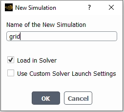
A new simulation folder will be created in the Project View, and the grid.cas file will be imported.
Enable to expose advanced features.
File
→ Preferences...
→ Icing → 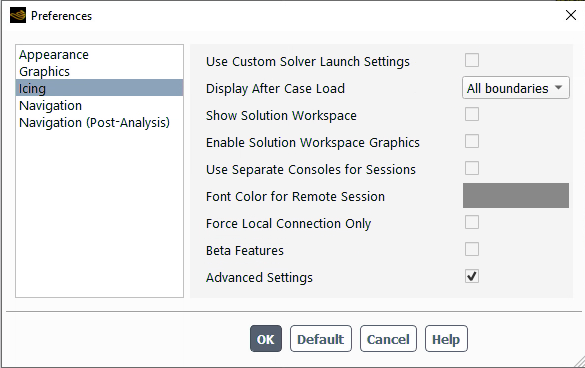
After the .cas file has been successfully loaded, a new Outline View tree appears under grid (loaded).
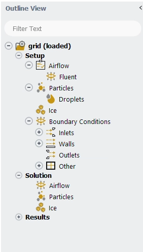
The mesh is now displayed in the Graphics window to the right.
Define the Simulation Type.
Setup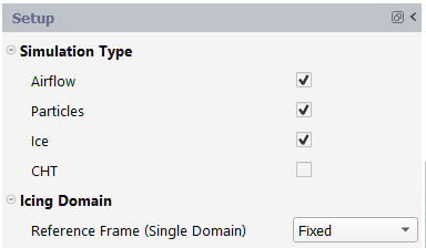
Enable and and under Simulation Type.
In the Icing Domain section, retain the following setting:
for Reference Frame (Single Domain).
Set the Airflow properties for the simulation.
Setup → Airflow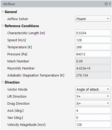
In the General section:
Retain the default selection of for Airflow Solver.
In the Reference Conditions section, retain the following settings:
0.5334for Characteristic Length [m].128for Speed [m/s].268for Temperature [K].84312for Pressure [Pa].
In the Direction section, retain the following settings:
for Vector Mode.
for Lift Direction.
for Drag Direction.
4for AoA [deg.].0for Yaw [deg.].128for Vector Magnitude [m/s].
Set the Fluent properties for the simulation.
Setup →
Airflow →
Fluent
In the Solver section:
Retain the default selection of for Type.
In the Models section, retain the following settings:
Enable .
for Turbulence.
for k-omega Model.
for Transition Model.
Enable both Viscous Heating and Turb. Production Limiter.
In the Materials section, retain the following setting:
for Fluid.
Set the Particles properties of the simulation.
Setup → Particles
Enable under Type.
Set the Droplets properties of the simulation.
Setup → Particles → Droplets
In the Droplet Conditions section, retain the following settings:
0.0024for LWC [kg/m3].20for Droplet Diameter [microns].1000for Water Density [kg/m3].Disable .
for Appendix Conditions.
In the Particles Distribution section, retain the following setting:
for Particles Distribution.
In the Model section, retain the following settings:
for Droplet Drag Model.
Set the Ice properties of the simulation.
Setup → Ice
In the Ice Accretion Conditions section, retain the following settings:
0.9for Recovery Factor.Disable Specify Icing Air Temperature.
100for Relative Humidity.
In the Model section, retain the following settings:
for Icing Model.
Enable Beading.
for Ice Shedding.
In the Ice Properties section, retain the following settings:
for Ice Density Type.
917for Constant Ice Density [kg/m3].
Set the Boundary Conditions for your simulation.
Setup → Boundary
Conditions → Inlets → pressure-far-field-11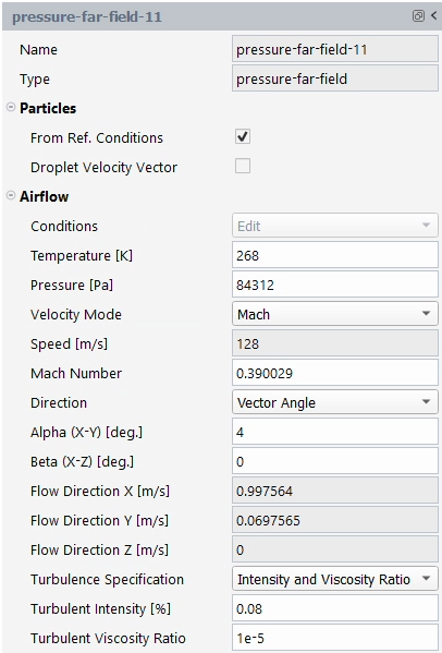
In the Airflow section:
Press to import the reference conditions of the case file.
Select under the Direction drop-down list.
0.997564for Flow Direction X.0.0697565for Flow Direction Y.0for Flow Direction Z.Select under the Turbulence Specification drop-down list.
0.08for Turbulent Intensity [%].1e-5for Turbulent Viscosity Ratio.Note: Repeat the steps above for pressure-far-field-4.
Setup → Boundary
Conditions → Walls → zone2000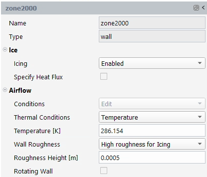
In the Airflow section:
Retain the default selection of for Thermal Conditions.
Press on to ensure a temperature value (adiabatic temperature + 10 degree) is imposed on the wall.
Select under the Wall Roughness drop-down list.
Set Roughness Height [m] to
0.0005.Repeat the steps above for zone2001 through zone2004.
Set the Solution properties of your simulation.
Solution → Airflow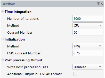
In the Time Integration section:
Set Number of Iterations to
1000.Select under the Method drop-down list.
Retain the default value of
50for Courant Number.
In the Initialization section:
Select under the Method drop-down list.
Retain the default value of
0.75for FMG Courant Number.
In the Post-processing Output section:
Retain the default selection of for Write Post-processing Files.
- Solution → Particles
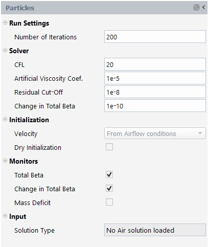
In the Run Settings section, retain the following setting:
200for Number of Iterations.
In the Solver section, retain the following settings:
20for CFL.1e-5for Artificial Viscosity Coef.1e-8for Residual Cut-Off.1e-10for Change in Total Beta.
In the Initialization section, retain the following settings:
The Velocity settings will be set to . The settings imported under the Airflow panel will be used.
Disable .
In the Monitors section, retain the following settings:
Enable .
Enable .
Disable .
- Solution → Ice
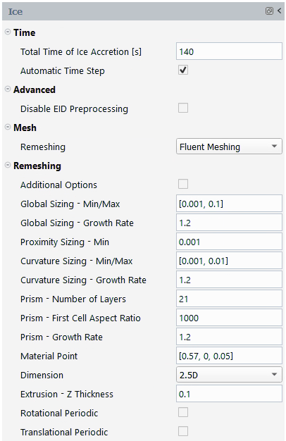
In the Time section, retain the following setting:
140for Total Time of Ice Accretion [s].Enable Automatic Time Step.
In the Mesh section:
Retain the default selection of for Remeshing.
In the Remeshing section, retain the following settings:
[0.001, 0.1]for Global Sizing - Min/Max.1.2for Global Sizing - Growth Rate.0.001for Proximity Sizing - Min.[0.001, 0.01]for Curvature Sizing - Min/Max.1.2for Curvature Sizing - Growth Rate.21for Prism - Number of Layers.1000for Prism - First Cell Aspect Ratio.1.2for Prism - Growth Rate.[0.57, 0, 0.05]for Material Point.for Dimension.
0.1for Extrusion - Z Thickness.
Open the ice_parametric.csv file found within fluent_icing_run_sequence.zip.
The file contains mandatory columns consisting of specific keywords listed below pertaining to settings within the Fluent Icing user interface Properties panel.
Cell A2 -
simulation: The .cas file used for the simulation.Cell B2 -
run: The run name which will be displayed within the Project View after the simulation completes.Cell C1 -
keywords: The solver used for the specific run.Cell C2 -
solverCell D2 -
PressureCell E2 -
Temperature
Cell F1 -
WallsCell F2 -
Temperature
Cell G1 -
Setup
                                            Particles
Cell G2 -
Droplet
                                                  Diameter
Cell H1 -
Setup
                                            Particles
Cell H2 -
LWC
The first run (flow_268K - B3) is a flow simulation at 5000 feet with a -10 degree temperature deviation from standard atmosphere. The walls are at adiabatic temperature +10 degrees.
Note: The Pressure and Temperature columns will overwrite everywhere you have Pressure or Temperature defined in Fluent Icing (Reference Values, Inlets, Walls). For example, Temperature will overwrite Temperature [K] (temperature at the wall) found under
Setup → Boundary
Conditions → Walls → zone2000.
Therefore, columns using the Walls keyword
have been added to use a different temperature at the
walls.Review the Particles and Ice runs.
Following Appendix C conditions,
20microns (Cell G4) is specified as your Droplet Diameter and0.0024kg/m3 (Cell H4) as the LWC. These settings match those found under the Droplets panel.Row 5 contains your Ice run as shown in the figure above.
You would continue adding the same Particles and Ice conditions for
30and40microns with a LWC of0.0017and0.00063respectively.
The same steps are repeated for 10,000ft (flow_258K) and 15,000ft (flow_248K).
The final spreadsheet is shown below:
Save this spreadsheet within your Run_Sequence_Tutorial.cffdb/grid project folder.
Launch the run sequence.
File → Read Run
Sequence...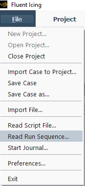
Select the ice_parametric.csv file from the Select File dialog. Press .
A dialog will open advising you Fluent Icing will now execute 21 runs in sequence. Press to proceed.
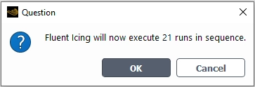
Once the computation is complete, the solution files will be written inside the Project View:
grid
flow
particles
ice
Project → Project
View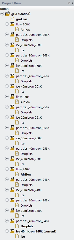
Under the grid (loaded) simulation, a list of run folders now appear. Expand each folder by clicking the + icon to show the files associated with the run. Each folder contains either an Airflow run, three Droplets runs, at different microns (20, 30, 40) and three Ice runs, also at different microns (20, 30, 40).
When reviewing the convergence of each run, you can see that the least ideal conditions are at 258 K and 20 microns.
To view the final ice shape, right-click Ice located under ice_20micron_258k within the Project View. Select → . Choose in the View Ice dialog.
Load the ice_20micron_258K settings.
Project View
→ ice_20micron_258K
Define the multi-shot run settings.
Solution → Ice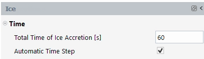
In the Time section, retain the following settings:
60for Total Time of Ice Accretion [s].Enable .
Press on to enable remeshing using Fluent Meshing.
Launch the simulation.
Solution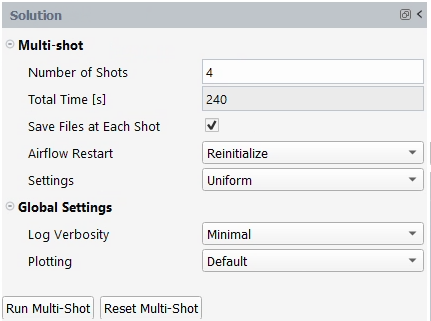
In the Multi-shot section, retain the following settings:
4for Number of Shots.Enable .
for Airflow Restart.
for Settings.
In the Global Settings section, retain the following settings:
for Log Verbosity.
for Plotting.
Launch the simulation by pressing .
A New run window will appear. Set the Name of the new run to
multishot_ice_parametricand press .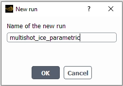
Note: Alternatively, you can launch the multi-shot calculation using
Solution Run
Multi-ShotOnce your multi-shot simulation ends, save your case.
Project
→ Simulation → Save
CaseOnce your case has been saved, close your simulation.
Project
→ Simulation
→ Close SimulationA Information dialog will open asking if you would like to save the case before closing the solver. Press to proceed.
Close your project.
Project
→ Project
→ CloseProceed with creating a new project file.
File → New
Project...
Enter
Run_Sequence_Tutorial_Iced_Gridas the Project file name within the Select File dialog.Select and import the grid.05.cas file found under Run_Sequence_Tutorial.cffdb/grid/multishot_ice_parametric/grid.05.cas.
Project → Import
CaseA New Simulation window will appear. Enter the Name of the New Simulation as
iced_grid, and check to enable . Click .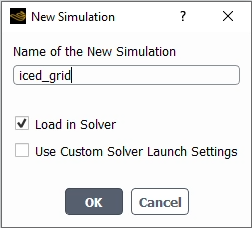
An Information dialog opens advising you of different node mapping between the current grid and previous solution files. Press to proceed since you will be creating new solution files based on the newly imported grid.
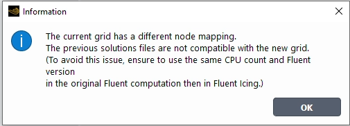
After the grid.05.cas file has been successfully loaded, a new Outline View tree appears under iced_grid (loaded).
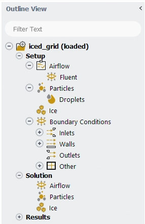
After importing the file, have a look at the pressure and temperature values under
Setup → AirflowIn the Reference Conditions section, retain the following settings:
258for Temperature [K].69691for Pressure [Pa].
Set the Boundary Conditions for your simulation.
Setup → Boundary
Conditions → Inlets → pressure-far-field-11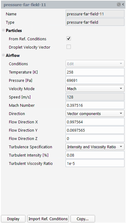
In the Airflow section:
Press to import the reference conditions of the case file.
Note: Repeat the steps above for pressure-far-field-4.
Setup → Boundary
Conditions → Walls → zone2000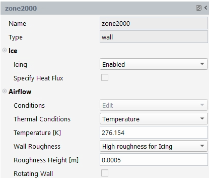
In the Airflow section:
Retain the default selection of for Thermal Conditions.
Press on to ensure a temperature value (adiabatic temperature + 10 degrees) is imposed on the wall.
Repeat the steps above for zone2001 through zone2004.
Save your case.
Project
→ Simulation → Save
CaseOnce your case has been saved, close your simulation.
Project
→ Simulation
→ Close SimulationA Information dialog will open asking if you would like to save the case before closing the solver. Press to proceed.
While in the same project, select and import the grid.cas input grid once again.
Project
→ Simulation → Import
Case
A New Simulation window will appear. Enter the Name of the New Simulation as
clean_grid, and check to enable . Click .
A new simulation folder will be created in the Project View and the grid.cas file will be imported.
Set the Airflow properties for the simulation.
Setup → Airflow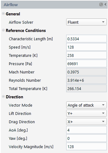
In the General section:
Retain the default selection of for Airflow Solver.
In the Reference Conditions section, retain the following settings:
0.5334for Characteristic Length [m].128for Speed [m/s].258for Temperature [K].69691for Pressure [Pa].
In the Direction section, retain the following settings:
for Vector Mode.
for Lift Direction.
for Drag Direction.
4for AoA [deg.].0for Yaw [deg.].128for Vector Magnitude [m/s].
Set the Boundary Conditions for your simulation.
Setup → Boundary
Conditions → Inlets → pressure-far-field-11In the Airflow section:
Press to import the reference conditions of the case file.
Note: Repeat the steps above for pressure-far-field-4.
Setup → Boundary
Conditions → Walls → zone2000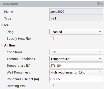
In the Airflow section:
Retain the default selection of for Thermal Conditions.
Press on to ensure a temperature value (adiabatic temperature + 10 degrees) is imposed on the wall.
Repeat the steps above for zone2001 through zone2004.
Save your case.
Project
→ Simulation → Save
CaseClose Fluent Icing.
File
→ Exit
A dialog will open asking you to save the clean_grid simulation case, press to proceed.
Reopen Fluent Icing, by selecting Icing, keeping Solver Processes at
4and pressing .Open your Run_Sequence_Tutorial_Iced_Grid project.
Project Library
→ Run_Sequence_Tutorial_Iced_Grid
Load your clean_grid project.
Project View
→ clean_grid
Open the perf_degradation.csv file found within fluent_icing_run_sequence.zip. You will notice a range of angles of attack. The goal of this .csv file is to run a sweep across various angles of attack using the imported grids and looking at the final performance degradation of the contaminated wing.
Two simulation are included in the angle of attack sweep, the clean_grid and iced_grid simulation. Each consists of six sweeps, using specific keywords found within Fluent Icing's Properties panels.
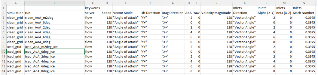
Review the various keywords and column titles. When ready, save this spreadsheet to your Run_Sequence_Tutorial_Iced_Grid.cffdb project folder.
Launch the run sequence.
File → Read Run
Sequence...Select the perf_degradation.csv file from the Select File dialog. Press .
A dialog will open advising you Fluent Icing will now execute 12 runs in sequence. Press to proceed.
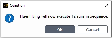
Once the computation is complete, the solution files will be written inside the Project View.
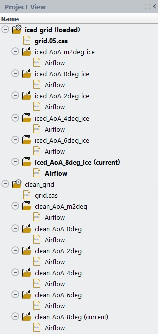
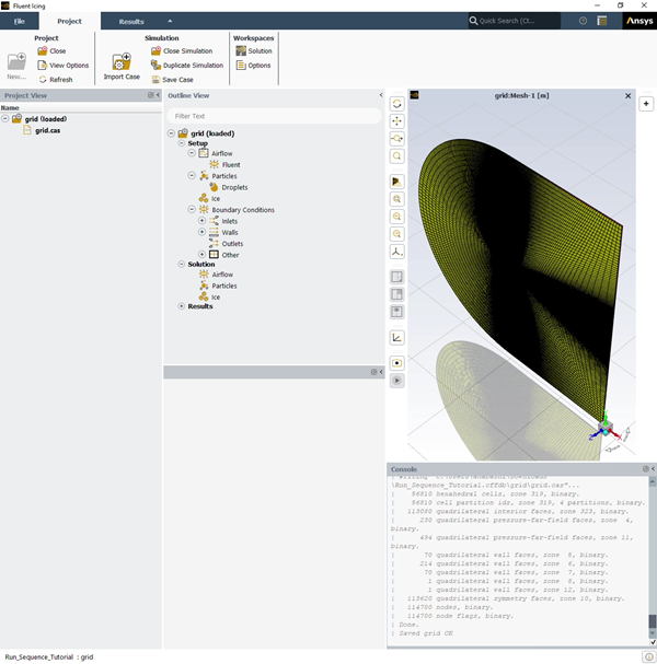
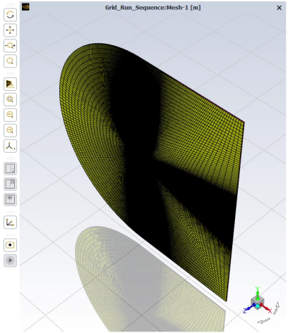
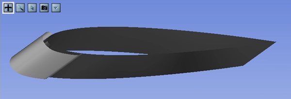
You can verify the convergence of each Airflow run. You will notice that the iced grid related to angles of attack 4, 6 and 8 have not converged well.
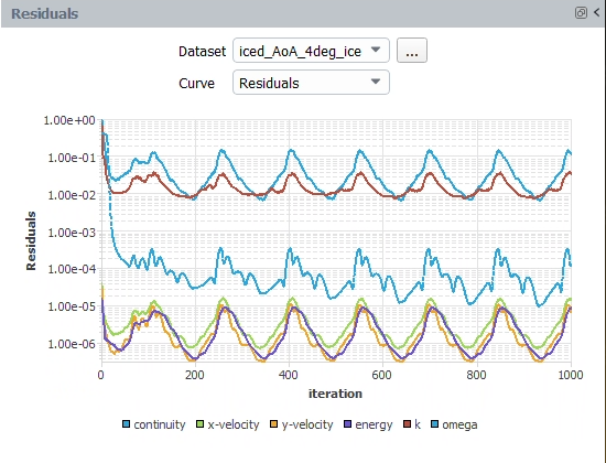
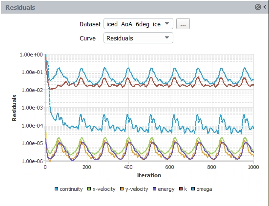
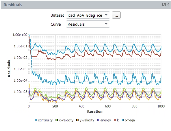
You can rerun them using the following new settings:
Solution → AirflowIn the Time Integration section:
3000for Number of Iterations.5for Courant Number.
File → Read Run
Sequence...Use the same perf_degradation.csv file to rerun this sequence.
Fluent Icing will detect that some runs already exist, click and select iced_AoA_4deg, iced_AoA_6deg and iced_AoA_8deg to be the only ones to rerun.
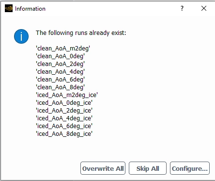
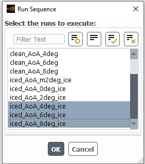
Press to proceed.
Once the simulation has ended, you can extract lift coefficient from each simulation by selecting the Airflow solution of each run and selecting
. Select
from the Curve drop-down and extract the value
at 1000iterations.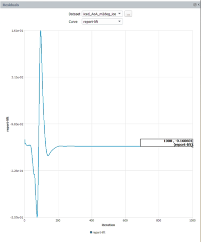
Note: Repeat the steps above for the other Airflow solutions found under iced_grid and clean_grid. Use the lift_vs_aoa.xlsx file found within fluent_icing_run_sequence.zip to plot your results.
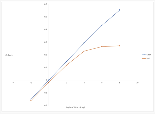
This tutorial demonstrated how to use Fluent Icing's Run Sequence feature to allow you to find out the most critical icing condition, generate an ice shape in that condition and compare the wing performance degradation due to ice at different angles of attack. The Run Sequence can be used for different usages. It is able to modify any settings in the Outline View hence why parametric studies can be performed for every property in Fluent Icing.
The following sections of this tutorial are:
This tutorial is divided into the following sections:
The objective of this tutorial is to simulate 3D droplet impingement on a realistic airplane configuration using Fluent Icing. Next you will cover the SLD (supercooled large droplets) regime where the large droplets can break-up, splash, and bounce based on their size and impact velocity, changing the collection efficiency distribution.
This tutorial demonstrates the droplet impingement computation over the DLR-F6 aircraft (wing/body) geometry. There is no yaw angle and the grid only contains one side of the symmetry plane. The grid is unstructured, composed of 4.8 million cells approximately.
This tutorial is written with the assumption that you have completed the introductory tutorials found in this manual and that you are familiar with the Ansys Fluent Outline View and Ribbon structure, see The Outline View and The Ribbon for more details. Some steps in the setup and solution procedure will not be shown explicitly.
The aircraft considered is the DLR-F6 which is a wing-body configuration. The flight condition used in this tutorial represents example of an in-flight icing condition. The problem considers the droplet impingement simulation over the aircraft’s wall boundaries. The grid is unstructured, composed of 4.8 million cells approximately. This mesh is very coarse, and therefore should be used for demonstration purposes only. The limits of the computational domain are defined by a hemispherical boundary defined as a pressure-far-field boundary type, and a flat circular boundary defined as a symmetry plane in the Z-direction.
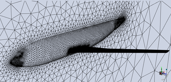
The following sections describe the setup and solution steps for this tutorial:
To prepare for running this tutorial:
Download the fluent_icing_droplet_impingement.zip file here .
Unzip fluent_icing_droplet_impingement.zip to your working directory.
The file, DLR.cas.h5, can be found in the folder.
Use the Fluent Launcher to start Ansys Fluent.
In the Fluent Launcher, set the Capability Level to Enterprise, then select Icing.
Set Solver Processes between
4and16.Click Start.
Alternatively, Fluent Icing can be opened using the icing (on Linux) or icing.bat (on Windows) file inside the fluent/bin/ folder.
Uncheck , , and .
Project
→ Workspaces →
Options
Create a new project file.
File
→ New...
Enter
Droplet_Impingement_Complete_Aircraftas the Project file name within the Select File dialog.Select and import the DLR.cas.h5 input grid.
Project
→ Simulation → Import
Case
A New Simulation window will appear. Enter the Name of the New Simulation as
DLR, and check to enable . Click .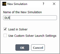
A new simulation folder will be created in the Project View, and the DLR.cas.h5 file will be imported.
After the .cas.h5 file has been successfully loaded, a new Outline View tree appears under DLR (loaded).
The mesh is now displayed in the Graphics window to the right.
Define the Simulation Type.
Setup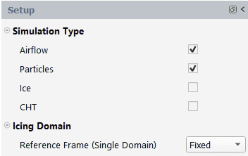
Enable and and disable under Simulation Type.
Set the Airflow properties of the simulation.
Setup → Airflow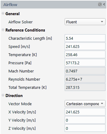
In the General section, retain the following setting:
for Airflow Solver.
In the Reference Conditions section, retain the following settings:
5.54for Characteristic Length [m].241.625for Speed [m/s].258.46for Temperature [K].57173.2for Pressure [Pa].
In the Direction section, retain the following settings:
for Vector Mode.
241.625for X Velocity [m/s].0for Y Velocity [m/s].0for Z Velocity [m/s].
Set the Solution properties of the simulation.
Solution → Airflow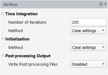
In the Time Integration section, retain the following setting:
200for Number of Iterations.for Method.
In the Initialization section, retain the following setting:
for Method.
In the Post-processing Output section, retain the following setting:
for Write Post-processing Files.
Launch the simulation.
Solution → Airflow → CalculateA New run window will appear. Set the Name of the new run to
airflow.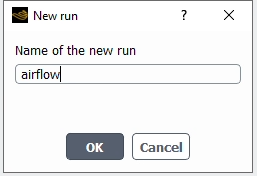
Once the computation is complete, the Airflow solution file will be written inside the new run directory, dlr/airflow.
Set the Particles properties of the simulation.
Setup → Particles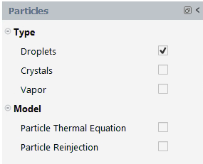
Enable under Type.
Set the Droplets properties of the simulation.
Setup → Particles → Droplets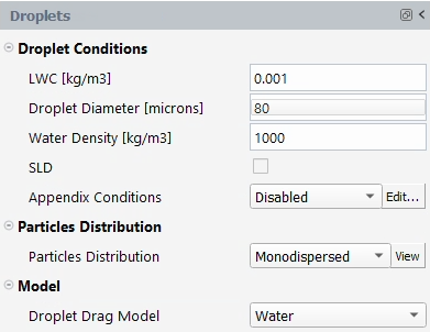
In the Droplet Conditions section, retain the following settings:
0.001for LWC [kg/m3].80for Droplet Diameter [microns].1000for Water Density [kg/m3].Disable .
for Appendix Conditions.
In the Particles Distribution section, retain the following setting:
for Particles Distribution.
In the Model section, retain the following setting:
for Droplet Drag Model.
Set the Boundary Conditions of the simulation.
Setup → Boundary
Conditions → Inlets → pressure-far-field-4The inlet boundary condition, pressure-far-field-4, is based on the initial droplet velocity and reference liquid water content which are both defined by enabling .
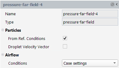
Set the Solution properties of the simulation.
Solution → Particles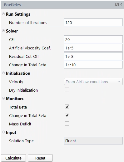
In the Run Settings section, retain the following setting:
120for Number of Iterations.
In the Solver section, retain the following settings:
20for CFL.1e-5for Artificial Viscosity Coef.1e-8for Residual Cut-Off.1e-10for Change in Total Beta.
In the Initialization section, retain the following settings:
The Velocity settings will be set to . The settings imported under the Airflow panel will be used.
Disable .
In the Monitors section, retain the following settings:
Enable .
Enable .
Disable .
Launch the simulation.
Solution → Particles → CalculateA New run window will appear. Set the Name of the new run to
particles.
Once the computation is complete, the Particles solution file will be written inside the new run directory, dlr/particles.
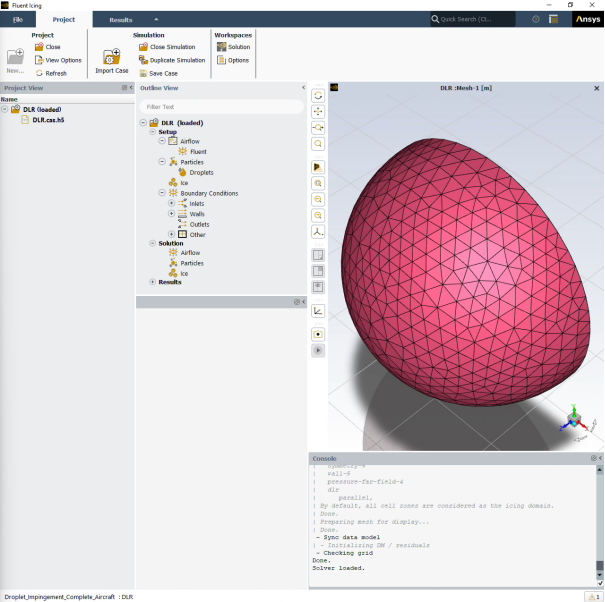
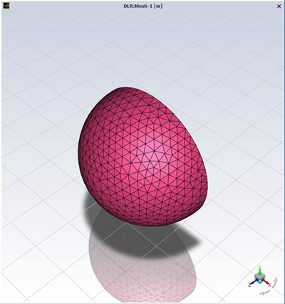
In this example, Fluent Icing will calculate for 120 iterations. Once the simulation finishes, you can view the collection efficiency distribution on the DLR-F6 aircraft.
Results
→ Quick-View →
Contour → 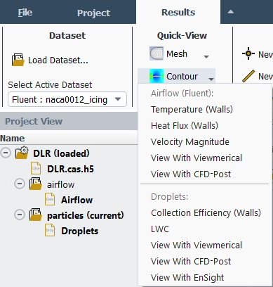
You can also use Viewmerical to view the collection efficiency plot.
Results
→ Quick-View →
Contour → Figure 1.51: Collection Efficiency Plots on the Wing Using Viewmerical: Root(Z=4m), Middle(Z=15m), Tip( Z=22.5m)
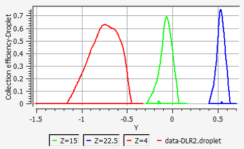
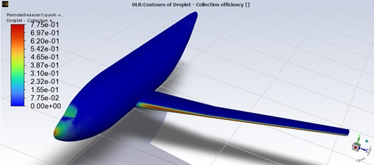
The peak in the collection efficiency increases towards the tip of the wing, due to the decrease in the thickness of the leading edge as the wing gets tapered. As mentioned in Langmuir-D Distribution, the droplets of same size are pushed away more by thicker sections of the aircraft, while thinner sections receive more of the same size droplets.
This tutorial is divided into the following sections:
This tutorial illustrates how to compute droplet impingement over a NACA23012 airfoil using the splashing and bouncing by post-processing model developed for Supercooled Large Droplets (SLD).
When the supercooled droplets are larger than 40 microns, they start to exhibit complex phenomena. They deform and break up into smaller droplets as they get close to aircraft surfaces, splash into smaller droplets upon impact that can be lost from the collection efficiency, and bounce off the surface if the local impingement angle is too shallow. To properly calculate collection efficiency for SLD, these phenomena should be accounted for.
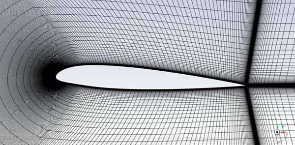
The following sections describe the setup and solution steps for this tutorial:
To prepare for running this tutorial:
Download the fluent_icing_droplet_impingement.zip file here .
Unzip fluent_icing_droplet_impingement.zip to your working directory.
The files, naca23012.cas.h5 and naca23012.dat.h5, can be found in the folder.
Use the Fluent Launcher to start Ansys Fluent.
In the Fluent Launcher, set the Capability Level to Enterprise, then select Icing.
Set Solver Processes between
4and16.Click Start.
Alternatively, Fluent Icing can be opened using the icing (on Linux) or icing.bat (on Windows) file inside the fluent/bin/ folder.
Uncheck , , and .
Project
→ Workspaces →
Options
Create a new project file.
File → New
Project...Enter
Splashing_Bouncing_Postprocessing_NACA23012as the Project file name within the Select File dialog.Select and import the naca23012.cas.h5 input grid.
Project
→ Simulation →
Import CaseA New Simulation window will appear. Enter the Name of the New Simulation as
naca23012,and check to enable and . Click .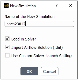
A new simulation folder will be created in the Project View, and the naca23012.cas.h5 file will be imported.
After the .cas.h5 file has been successfully loaded, a new Outline View tree appears under naca23012 (loaded).
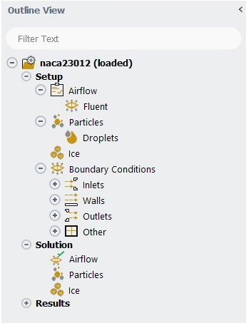
The mesh is now displayed in the Graphics window to the right.
Define the Simulation Type.
Setup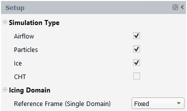
Enable and and disable under Simulation Type.
Set the Airflow properties of the simulation.
Setup → AirflowNote: In this tutorial, all airflow properties are automatically imported when loading the provided Fluent airflow solution input files, naca23012.cas.h5 and naca23012.dat.h5.
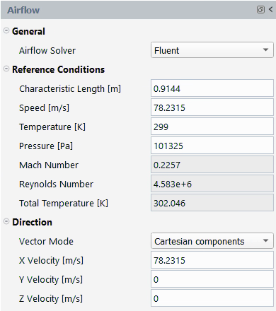
Set the Particles properties of the simulation.
Setup → ParticlesEnable under Type.
Set the Droplets properties of the simulation.
Setup → Particles → Droplets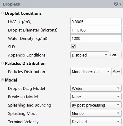
In the Droplet Conditions section, retain the following settings:
0.0005for LWC [kg/m3].111.106for Droplet Diameter [microns].1000for Water Density [kg/m3].Enable .
for Appendix Conditions.
In the Particles Distribution section, retain the following setting:
for Particles Distribution.
In the Model section, retain the following settings:
for Droplet Drag Model.
for Break-Up Model.
for Splashing and Bouncing.
for Splashing Model.
for Terminal Velocity.
Set the Boundary Conditions of the simulation.
Setup → Boundary
Conditions → Inlets → pressure-far-field-4The inlet boundary condition, pressure-far-field-4, is based on the initial droplet velocity and reference liquid water content which are both defined by enabling .
Set the Solution properties of the simulation.
Solution → Particles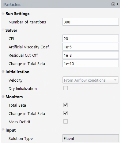
In the Run Settings section, retain the following setting:
300for Number of Iterations.
In the Solver section, retain the following settings:
20for CFL.1e-5for Artificial Viscosity Coef.1e-8for Residual Cut-Off.1e-10for Change in Total Beta.
In the Initialization section, retain the following settings:
The Velocity settings will be set to . The settings imported under the Airflow panel will be used.
Disable .
In the Monitors section, retain the following settings:
Enable .
Enable .
Disable .
Launch the simulation.
Solution → Particles → CalculateA New run window will appear. Set the Name of the new run to
particles-splashing-and-bouncing-on.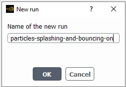
Once the computation is complete, the Particles solution file will be written inside the new run directory particles-splashing-and-bouncing-on/Droplets.
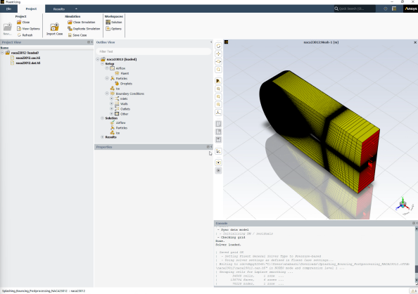
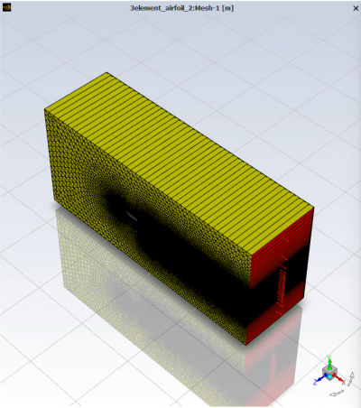
In this example, Fluent Icing will calculate for 300 iterations. Once the simulation finishes, you can view the collection efficiency distribution on the NACA23012.
Results
→ Quick-View →
Contour → 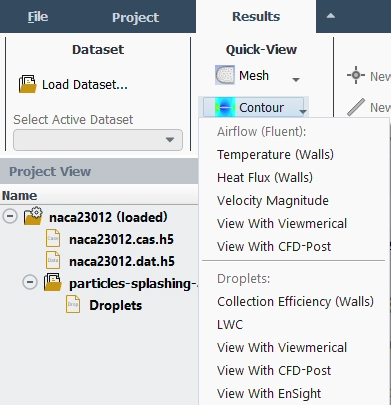
You can also use Viewmerical to view the collection efficiency plot.
Results
→ Quick-View →
Contour →
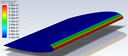
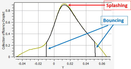
The graph above shows the difference in collection efficiency when splashing and bouncing are enabled by post processing. Splashing effects remove some collection at the stagnation point while bouncing removes collection past a certain chord-wise limit on the upper and lower surfaces.
Note: To obtain the curve without splashing and bouncing, a separate particles run should be performed by changing Splashing and Bouncing to .
![]() Setup → Particles → Droplets
Setup → Particles → Droplets
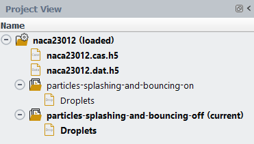
This tutorial is divided into the following sections:
This tutorial illustrates how to compute droplet primary impingement and re-impingement over the different components of a three-element airfoil using the splashing and bouncing model with external reinjection developed for Supercooled Large Droplets (SLD).
When supercooled droplets reach a size of 40 microns, they begin to display complicated behaviors. As they approach aircraft surfaces, they distort and break up into smaller droplets, splash into smaller droplets upon impact, which can reduce collecting efficiency, and bounce off the surface if the local impingement angle is too shallow. Small ejecta from splashing are reinjected into the airflow and can hit the surface again, enhancing collecting efficiency at this new site. A slat element (on the left), a main wing (in the middle), and a flap element (on the right) make up the three-element airfoil. Large droplets will strike the slat element, while the main and flap components will gather more droplets from the reinjection.
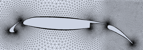
The following sections describe the setup and solution steps for this tutorial:
To prepare for running this tutorial:
Download the fluent_icing_droplet_reinjection.zip file here .
Unzip fluent_icing_droplet_reinjection.zip to your working directory.
The files, 3element_airfoil_2.cas.h5, 3element_airfoil_2.dat.h5 and distri.csv can be found in the folder.
Use the Fluent Launcher to start Ansys Fluent.
In the Fluent Launcher, set the Capability Level to Enterprise, then select Icing.
Set Solver Processes between
4and16.Click Start.
Alternatively, Fluent Icing can be opened using the icing (on Linux) or icing.bat (on Windows) file inside the fluent/bin/ folder.
Uncheck , , and .
Project
→ Workspaces →
Options
Create a new project file.
File → New
Project...Enter
Reinjection_Three_Element_Airfoilas the Project file name within the Select File dialog.Select and import the 3element_airfoil_2.cas.h5 input grid.
Project
→ Simulation →
Import CaseA New Simulation window will appear. Enter the Name of the New Simulation as
3element_airfoil_2,and check to enable and . Click .
A dialog will open asking you to set the operating pressure to 0 Pa. Press to not accept this change.
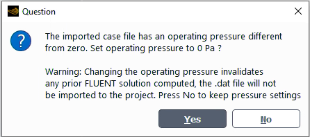
A new simulation folder will be created in the Project View, and the 3element_airfoil_2.cas.h5 file will be imported.
After the .cas.h5 file has been successfully loaded, a new Outline View tree appears under naca23012 (loaded).
The mesh is now displayed in the Graphics window to the right.
Define the Simulation Type.
SetupEnable and and disable under Simulation Type.
Set the Airflow properties of the simulation.
Setup → AirflowNote: In this tutorial, all airflow properties are automatically imported when loading the provided Fluent airflow solution input files, 3element_airfoil_2.cas.h5 and 3element_airfoil_2.dat.h5.
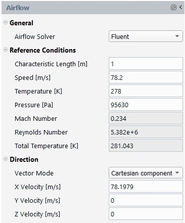
Set the Particles properties of the simulation.
Setup → ParticlesEnable under Type.
Set the Droplets properties of the simulation.
Setup → Particles → Droplets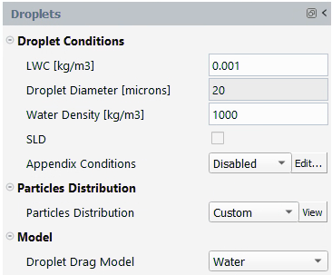
In the Droplet Conditions section, retain the following settings:
0.001for LWC [kg/m3].20for Droplet Diameter [microns].1000for Water Density [kg/m3].Disable .
for Appendix Conditions.
In the Particles Distribution section, retain the following setting:
for Particles Distribution.
Beside , click followed by and import the distri.csv file.
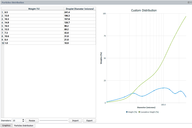
In the Model section, retain the following setting:
for Droplet Drag Model.
Set the Boundary Conditions of the simulation.
Setup → Boundary
Conditions → Inlets → pressure-far-field-4The inlet boundary condition, pressure-far-field-4, is based on the initial droplet velocity and reference liquid water content which are both defined by enabling .
Set the Solution properties of the simulation.
Solution → Particles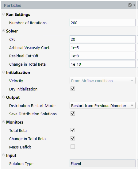
In the Run Settings section, retain the following setting:
200for Number of Iterations.
In the Solver section, retain the following settings:
20for CFL.1e-5for Artificial Viscosity Coef.1e-8for Residual Cut-Off.1e-10for Change in Total Beta.
In the Initialization section, retain the following settings:
The Velocity settings will be set to . The settings imported under the Airflow panel will be used.
Disable .
In the Output section, retain the following settings:
for Distribution Restart Mode.
Enable .
In the Monitors section, retain the following settings:
Enable .
Enable .
Disable .
Launch the simulation.
Solution → Particles → CalculateA New run window will appear. Set the Name of the new run to
droplets-no-sld.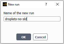
Once the computation is complete, the Particles solution file will be written inside the new run directory droplets-no-sld/Droplets and the Project View will be updated.
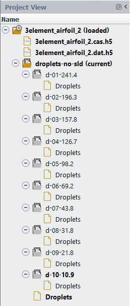
Go back to the Particles panel.
Setup → Particles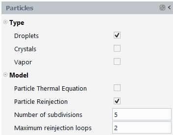
In the Model section, retain the following settings:
Enable .
5for .2.
Update the Droplets properties of the simulation.
Solution → Particles → Droplets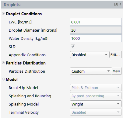
In the Model section, retain the following setting:
for .
Set the Boundary Conditions of the simulation.
Setup → Boundary
Conditions → Inlets → wall-5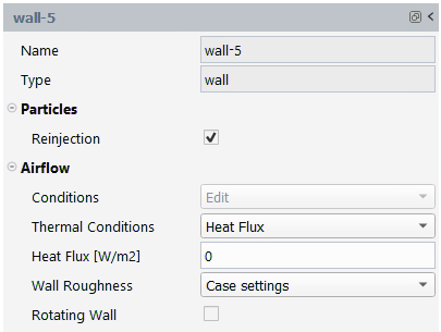
In the Particles section, retain the following setting:
Enable .
Note: Repeat this step for all walls (wall-6 through wall-15).
Update the Solution properties of the simulation.
Solution → Particles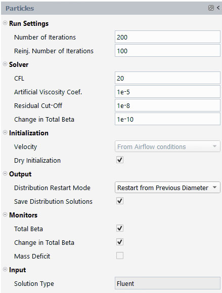
In the Run Settings section, retain the following setting:
200for Number of Iterations.100for Reinj. Number of Iterations.
Launch the simulation.
Solution → Particles → CalculateA New run window will appear. Set the Name of the new run to
droplets-reinjection.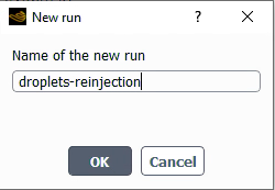
Once the computation is complete, the Particles solution file will be written inside the new run directory droplets-reinjection/Droplets and the Project View will be updated with both Primary-Droplets and Droplets files.
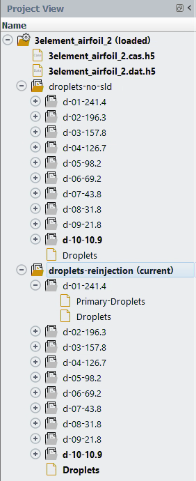
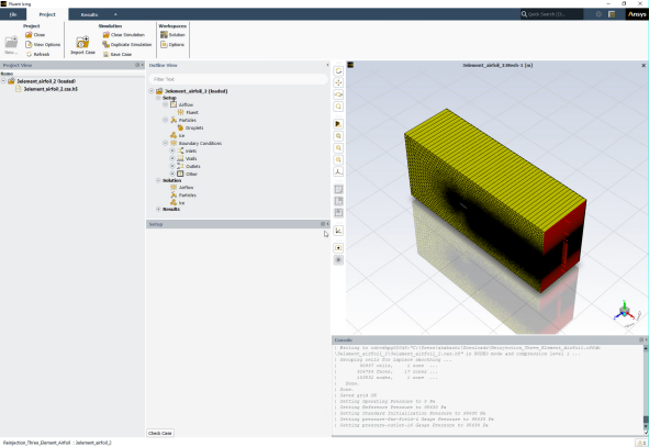
Compare the results of both combined solutions using Viewmerical.
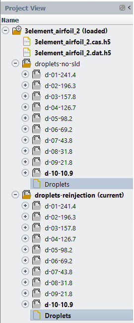
Right-click both Droplets file and select
Project
View → 3element_airfoil_2 → Droplets → Pick the two imported objects in Viewmerical's Objects panel and choose under Split screen.
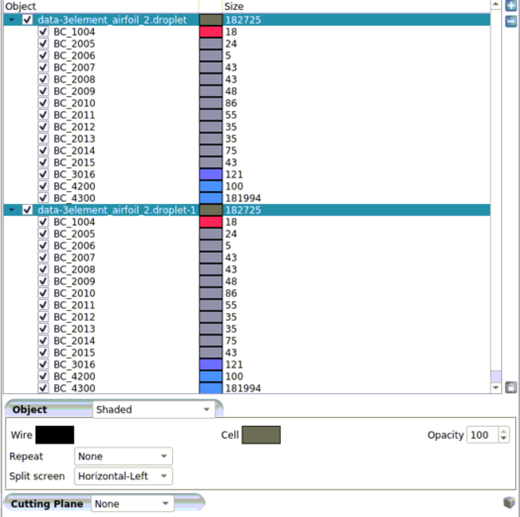
In the Data panel, select for Data, for Color range. Click on the Shared icon and change the maximum value to
0.0025kg/m3.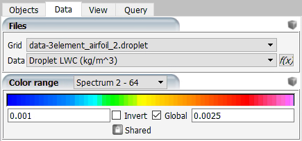
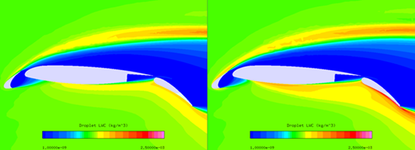
The image above shows the difference in LWC caused by considering (right) or without considering (left) droplet reinjection based on Wright's splashing model. When reinjection is considered, the droplet concentration on the pressure side of the flap element and the main wing increases.
In the Objects section, enable only the wall boundary conditions corresponding to the slat element (BC_2009, BC_2014) and keep both solutions selected.
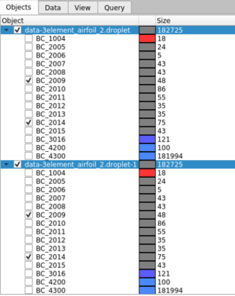
Plot the collection efficiency by by heading to the Data panel and selecting . In the Query panel, set 2D Plot to , Target to , Cutting plane to and in the drop-down list for the abscissa.
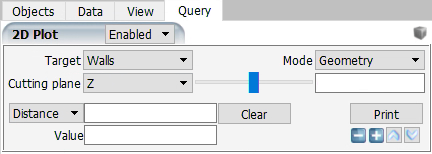
Adjust the color of the curves under Curve Settings (green for the full primary collection case and black for the reinjection case):
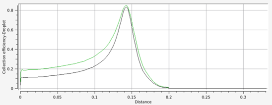
Repeat the same for the main wing (BC_2005, BC_2010, BC_2011, BC_2012, BC_2015).
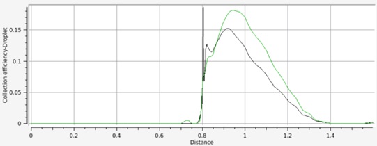
Repeat the same for the flap (BC_2006, BC_2007, BC_2008, BC_2013, ).
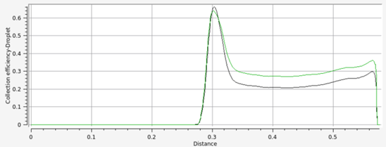
You can examine the outcomes on the slat, main, and flap elements from top to bottom. It emphasizes the differences between collecting all of the SLD at the wall and using a splashing model with reinjection. We can discern a peak displaying the mass collected after reinjection, especially on the major wing.
The following sections of this tutorial are:
This tutorial is divided into the following sections:
Icing calculations at high air speeds require special treatment when the total temperature of the flow is very close or above freezing temperature. This condition may arise when the icing temperature is low but the Mach number is in the mid- to transonic range. For these cases, an additional feature called Extended Icing Data (EID) will be used, where Fluent Icing performs additional pre-processing of the flow to improve the icing thermodynamics for this regime.
The problem considers the icing computations around a NACA0012 airfoil at an angle of attack of 7° and a free-stream Mach number of 0.5912 at low icing temperature. The ice shapes encountered in this flow regime, typically referred to as beak ice, are usually characterized by well-defined small horns growing at a short distance from the stagnation point on a mostly uncontaminated surface. This is a type of ice shape that is usually observed on the outboard sections of helicopter main rotor blades.
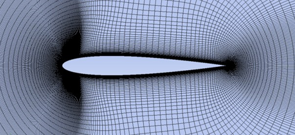
The following sections describe the setup and solution steps for this tutorial:
To prepare for running this tutorial:
Download the fluent_icing_ice_accretion.zip file here .
Unzip fluent_icing_ice_accretion.zip to your working directory.
The file, naca0012.cas.h5, can be found in the folder.
Use the Fluent Launcher to start Ansys Fluent.
In the Fluent Launcher, set the Capability Level to Enterprise, then select Icing.
Set Solver Processes between
4and16.Click Start.
Alternatively, Fluent Icing can be opened using the icing (on Linux) or icing.bat (on Windows) file inside the fluent/bin/ folder.
Uncheck , , and .
Project
→ Workspaces →
Options
Create a new project file.
File
→ New...
Enter
Ice_Accretion_High_Speedas the Project file name within the Select File dialog.Select and import the naca0012.cas.h5 input grid.
Project
→ Simulation → Import
Case
A New Simulation window will appear. Enter the Name of the New Simulation as
naca0012, and check to enable . Click .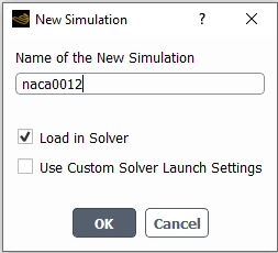
A new simulation folder will be created in the Project View, and the naca0012.cas.h5 file will be imported.
After the .cas.h5 file has been successfully loaded, a new Outline View tree appears under naca0012 (loaded).
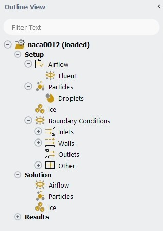
The mesh is now displayed in the Graphics window to the right.
Define the Simulation Type.
Setup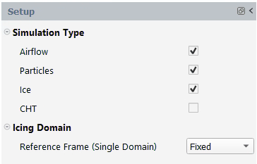
Enable and and under Simulation Type.
Set the Airflow properties of the simulation.
Setup → Airflow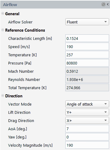
In the General section, retain the following setting:
for Airflow Solver.
In the Reference Conditions section, retain the following settings:
0.1524for Characteristic Length [m].190for Speed [m/s].257for Temperature [K].80800for Pressure [Pa].
In the Direction section, retain the following settings:
for Vector Mode.
for Lift Direction.
for Drag Direction.
7for AoA [deg.].0for Yaw [deg.].190for Velocity Magnitude [m/s].
Set the Fluent properties of the simulation.
Setup → Fluent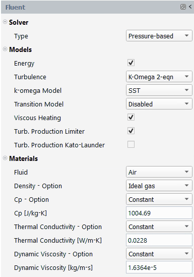
In the Solver section, retain the following setting:
for Type.
In the Models section, retain the following settings:
Enable Energy.
for Turbulence.
for k-omega Model.
for Transition Model.
Enable Viscous Heating.
Enable Turb. Production Limiter.
In the Materials section, retain the following settings:
for Fluid.
for Density - Option.
for Cp - Option.
1004.69for Cp [J/kg-K].for Thermal Conductivity - Option.
0.0228for Thermal Conductivity [W/m-K].for Dynamic Viscosity - Option.
1.6364e-5for Dynamic Viscosity [kg/m-s].
Set the Particles properties of the simulation.
Setup → ParticlesEnable under Type.
Set the Droplets properties of the simulation.
Setup → Particles → Droplets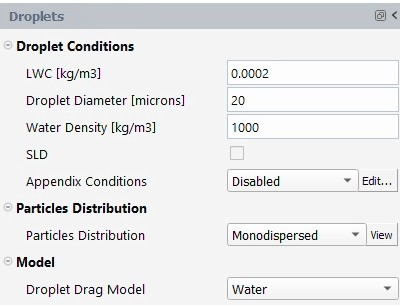
In the Droplet Conditions section, retain the following settings:
0.0002for LWC [kg/m3].20for Droplet Diameter [microns].1000for Water Density [kg/m3].Disable .
for Appendix Conditions.
In the Particles Distribution section, retain the following setting:
for Particles Distribution.
In the Model section, retain the following setting:
for Droplet Drag Model.
Set the Ice properties of the simulation.
Setup → Ice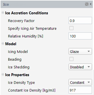
In the Ice Accretion Conditions section, retain the following settings:
0.9for Recovery Factor.Disable Specify Icing Air Temperature.
100for Relative Humidity.
In the Model section, retain the following settings:
for Icing Model.
Disable Beading.
for Ice Shedding.
In the Ice Properties section, retain the following settings:
for Ice Density Type.
917for Constant Ice Density [kg/m3].
Set the Boundary Conditions of the simulation.
Setup → Boundary
Conditions → Inlets → pressure-far-field-4The inlet boundary condition, pressure-far-field-4, is based on the initial droplet velocity and reference liquid water content which are both defined by enabling .
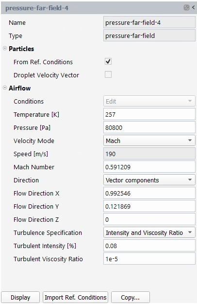
Press on to import the reference conditions of the case file. All reference conditions are now imported to your boundary condition.
In the Particles section, retain the following settings:
Enable From Ref. Conditions.
Disable Droplet Velocity Vector.
In the Airflow section, retain the following settings:
257for Temperature [K].80800for Pressure [Pa].for Velocity Mode.
0.591209for Mach Number.for Direction.
0.992546for Flow Direction X.0.121869for Flow Direction Y.0for Flow Direction Z.for Turbulence Specification.
0.08for Turbulent Intensity [%].1e-5for Turbulent Viscosity Ratio.
Setup → Boundary
Conditions → Walls → wall-5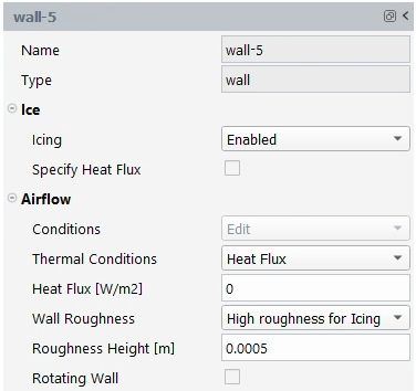
In the Ice section, retain the following setting:
for Icing.
In the Airflow section, retain the following settings:
for Thermal Conditions.
0for Heat Flux [W/m2].For the EID calculations, icing walls need to be set as adiabatic walls. Heat transfer coefficients will be extracted later on as part of EID solution.
for Wall Roughness.
0.0005for Roughness Height [m].Repeat the steps above for wall-6 and wall-7.
Setup → Boundary
Conditions → Walls → wall-8In the Ice section, retain the following setting:
for Icing.
Note: Sink boundaries eliminate impingement and runback while also preventing ice formation. In this case, you'll use it to keep runback water from reaching the lower side's trailing edge.
Set the Solution properties of the simulation.
Solution → Airflow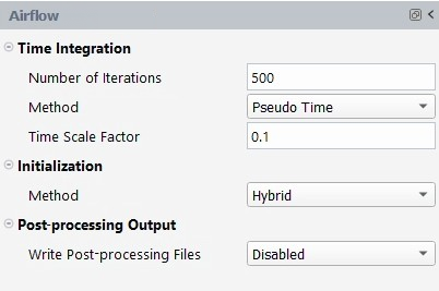
In the Time Integration section, retain the following settings:
500for Number of Iterations.for Method.
0.1for Time Scale Factor.Note: Time Scale Factor is a case specific setting and may need to be reduced for stability or increased for computational efficiency.
In the Initialization section, retain the following setting:
for Method.
In the Post-processing Output section, retain the following setting:
for Write Post-processing Files.
Solution → Particles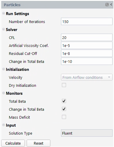
In the Run Settings section, retain the following setting:
150for Number of Iterations.
In the Solver section, retain the following settings:
20for CFL.1e-5for Artificial Viscosity Coef.1e-8for Residual Cut-Off.1e-10for Change in Total Beta.
In the Initialization section, retain the following settings:
The Velocity settings will be set to . The settings imported under the Airflow panel will be used.
Disable .
In the Monitors section, retain the following settings:
Enable .
Enable .
Disable .
Solution → Ice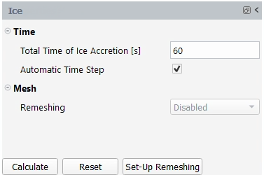
In the Time section, retain the following setting:
60for Total Time of Ice Accretion [s].Enable Automatic Time Step.
Launch the simulation.
Solution → Airflow → CalculateA New run window will appear. Set the Name of the new run to
flow.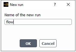
Once
flowis complete, follow the steps below. Solution → Particles → CalculateA New run window will appear. Set the Name of the new run to
particles.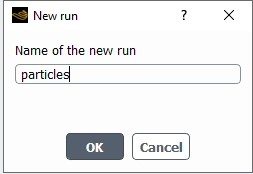
Once
particlesis complete, follow the steps below. Solution → Ice → CalculateA New run window will appear. Set the Name of the new run to
ice.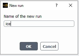
Once the computation is complete, the solution files will be written inside the new run directory:
naca0012
flow
particles
ice
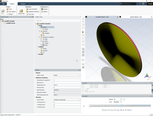
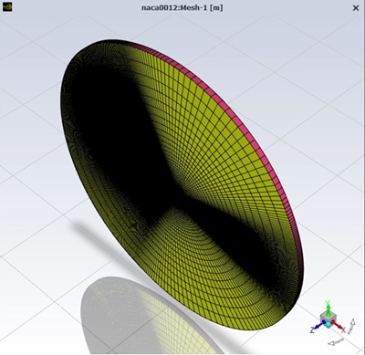
In this example, Fluent Icing will calculate the airflow, particles and ice simulation. Once the simulation finishes, you can view the liquid water content on the NACA0012 airfoil.
Results
→ Quick-View →
Contour →
You can also use Viewmerical to view the ice cover.
Results
→ Quick-View →
Ice Cover → Ice Cover -
Viewmerical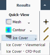
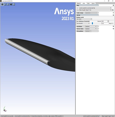
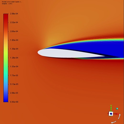
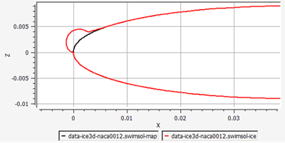
This tutorial is divided into the following sections:
Ice that accretes on rotating components like helicopter rotors, propellers, and engine fan blades can shed due to breakup under centrifugal forces. When shedding happens asymmetrically, rotors experience vibrations which can be severe. Estimating when and how much ice will shed from a rotor blade can help establish part of the parameters needed to analyze rotor vibrations and structural analysis. The ice shedding feature is designed for the purpose of reporting the amount of ice mass that shed during icing under the influence of rotational forces.
To compute ice delamination from the substrate and ice cracking, the ice volume is meshed internally by ICE3D using the same surface mesh topology as the substrate. A stress analysis is then performed. This operation takes place at a user-specified frequency which coincides with the solution output of ICE3D. The stress analysis may reveal that multiple ice fragments delaminate and crack. These fragments are reported in the log and the lost ice mass is removed from the solution. Icing time steps for engine fans usually range between 1e-7 to 1e-4 seconds, while the stress analysis interval can be set much higher, around 0.5 – 2 seconds.
For more details on the ice shedding model, consult Fluent User's Guide and Ansys FENSAP-ICE User Manual.
In this version, the stress analysis of the ice is done using a single CPU only. Large surface grids of helicopter rotors and turbo-prop blades may take a long time to complete a single stress analysis. Engine fan and rotor blades are more suited for use with the current version of the ice shedding implementation.
Non-conformal rotational periodicity is not supported in Fluent Icing. The periodic boundaries on either side need to be perfectly node-to-node matching.
Ice stress analysis is done on single shot ice shapes, with the ice volume mesh created as a single layer between the starting surface and the final ice shape. Multi-shot ice shapes and multi-shot workflows in general are not yet supported.
In this tutorial, the ice shedding feature uses a simple fan blade shown in the figure below. The structured computational mesh is 10-degree rotationally periodic. There is a tip gap between the shroud and the fan blade. The exit is split into two sections, one for the bypass flow and one for the engine core flow. The solution process will begin with airflow, followed with a particle solution for droplets, and finally with an ice solution to compute ice accumulation and shedding.
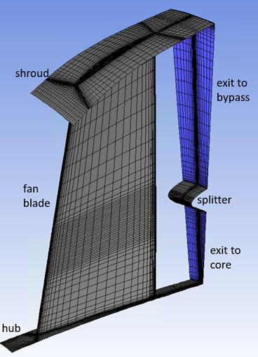
The following sections describe the setup and solution steps for this tutorial:
To prepare for running this tutorial:
Download the fluent_icing_ice_accretion.zip file here .
Unzip fluent_icing_ice_accretion.zip to your working directory.
The file, fan.cas.h5, can be found in the folder.
Use the Fluent Launcher to start Ansys Fluent.
In the Fluent Launcher, set the Capability Level to Enterprise, then select Icing.
Set Solver Processes between
4and16.Click Start.
Alternatively, Fluent Icing can be opened using the icing (on Linux) or icing.bat (on Windows) file inside the fluent/bin/ folder.
Uncheck , , and .
Project
→ Workspaces →
Options
Create a new project file.
File
→ New...
Enter
Ice_Shedding_on_Fanas the Project file name within the Select File dialog.Select and import the fan.cas.h5 input grid.
Project
→ Simulation → Import
CaseA New Simulation window will appear. Enter the Name of the New Simulation as
fan, and check to enable . Click .
A new simulation folder will be created in the Project View, and the fan.cas.h5 file will be imported.
Enable to expose advanced features.
File
→ Preferences...
→ Icing → After the .cas.h5 file has been successfully loaded, a new Outline View tree appears under fan (loaded).
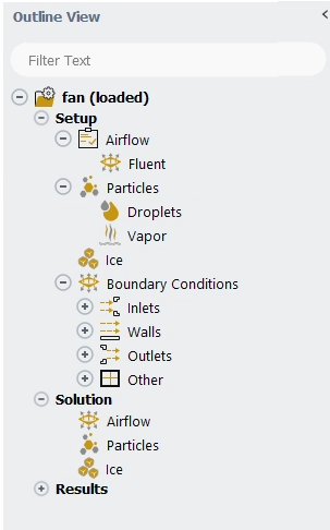
The mesh is now displayed in the Graphics window to the right.
Define the Simulation Type.
Setup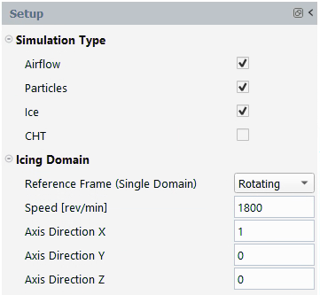
Enable and and under Simulation Type.
In the Icing Domain section, retain the following setting:
for Reference Frame (Single Domain).
1800for Speed [rev/min].1for Axis Direction X.0for Axis Direction Y.0for Axis Direction Z.
Set the Airflow properties of the simulation.
Setup → Airflow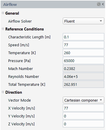
In the General section, retain the following setting:
for Airflow Solver.
In the Reference Conditions section, retain the following settings:
0.1for Characteristic Length [m].77for Speed [m/s].260for Temperature [K].65000for Pressure [Pa].
In the Direction section, retain the following settings:
for Vector Mode.
77for X Velocity [m/s].0for Y Velocity [m/s].0for Z Velocity [m/s].
Set the Fluent properties of the simulation.
Setup → Fluent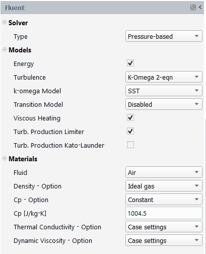
In the Solver section, retain the following setting:
for Type.
In the Models section, retain the following settings:
Enable Energy.
for Turbulence.
for k-omega Model.
for Transition Model.
Enable Viscous Heating.
Enable Turb. Production Limiter.
In the Materials section, retain the following settings:
for Fluid.
for Density - Option.
for Cp - Option.
1004.5for Cp [J/kg-K].for Thermal Conductivity - Option.
for Dynamic Viscosity - Option.
Set the Particles properties of the simulation.
Setup → Particles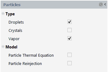
Enable and under Type.
Set the Droplets properties of the simulation.
Setup → Particles → Droplets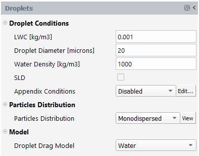
In the Droplet Conditions section, retain the following settings:
0.0001for LWC [kg/m3].20for Droplet Diameter [microns].1000for Water Density [kg/m3].Disable .
for Appendix Conditions.
In the Particles Distribution section, retain the following setting:
for Particles Distribution.
In the Model section, retain the following setting:
for Droplet Drag Model.
Set the Vapor properties of the simulation.
Setup → Particles → Vapor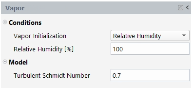
In the Conditions section, retain the following settings:
for Vapor Initialization.
100for Relative Humidity [%].
In the Model section, retain the following setting:
0.7for Turbulent Schmidt Number.
Set the Ice properties of the simulation.
Setup → Ice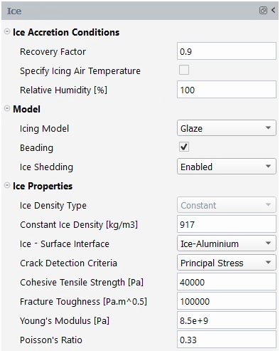
In the Ice Accretion Conditions section, retain the following settings:
0.9for Recovery Factor.Disable Specify Icing Air Temperature.
100for Relative Humidity.
In the Model section, retain the following settings:
for Icing Model.
Enable Beading.
for Ice Shedding.
In the Ice Properties section, retain the following settings:
for Ice Density Type.
917for Constant Ice Density [kg/m3].for Ice - Surface Interface.
for Crack Detection Criteria.
40000for Cohesive Tensile Strength [Pa].100000for Fracture Toughness [Pa.m^0.5].8.5e+9for Young's Modulus [Pa].0.33for Poisson's Ratio.
Note: The Relative Humidity setting here is ineffective when vapor model is activated as part of the particles simulation. The locally variable humidity on the wall will instead be provided by the vapor transport solution.
The Icing Model is set to as there will be increased aerodynamic heating from the root to the tip of the blade and conditions can change from rime to glaze towards the tip.
is enabled to find out the resulting ice surface roughness during ice accretion.
Ice shedding is enabled to compute ice stress and crack propagation as part of the simulation. Enabling this option will bring up a list of parameters that are used in the ice stress analysis. Currently only two options are supported for Ice – Surface Interface: and . This choice affects the normal and shear adhesive strength between the ice and the substrate.
Crack Detection Criteria can be set to either or . is usually used for ductile materials, while is better suited for brittle materials like ice. When is chosen, the critical stress for crack initiation and propagation will be the Cohesive Tensile Stress set in this panel.
Set the Boundary Conditions of the simulation.
Setup → Boundary
Conditions → Inlets → zone1004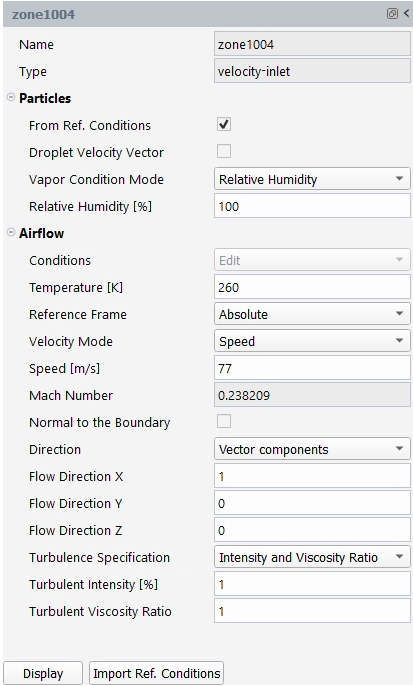
In the Particles section, retain the following settings:
Enable .
Note: When is checked, the LWC and droplet diameter values will be taken from the conditions defined in Droplets. Water vapor boundary condition at the inlet is set to 100% relative humidity which will apply the vapor saturation pressure at the air temperature set for this boundary.
Disable Droplet Velocity Vector.
for Vapor Condition Mode.
100for Relative Humidity [%].
In the Airflow section, retain the following settings:
for Conditions.
260for Temperature [K].for Reference Frame.
Note: The Reference Frame determines if the velocity components are declared in absolute or rotating frame of reference. In this case, the air is flowing straight in the X direction onto the fan, while the fan is rotating as part of the domain with it’s rotation set earlier in the Setup window. On the other hand, if you had an inlet attached to a rotating assembly with the air coming out of this inlet rotating with the same rate as the domain, then you would need to set the reference frame to relative.
for Velocity Mode.
77for Speed [m/s].for Direction.
1for Flow Direction X.0for Flow Direction Y.0for Flow Direction Z.for Turbulence Specification.
1for Turbulent Intensity [%].1for Turbulent Viscosity Ratio.Note: Turbulent intensity and viscosity ratio are set to 1 instead of quiescent flow since this is a fan domain and incoming flow could already have some turbulence in an actual situation.
Setup → Boundary
Conditions → Walls → zone2005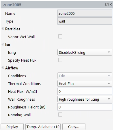
Note: All walls are to be set as adiabatic (heat flux = 0) with zero roughness. In turbomachinery icing problems, it is preferable to have zero surface roughness, allowing it to be built up with the beading model. Otherwise, this artificial roughness setting applied to all walls can strongly change flow dynamics.
In the Particles section, retain the following setting:
Disable Vapor Wet Wall.
In the Ice section, retain the following setting:
Note: To simplify the problem, only the fan blade and the splitter will be enabled for icing, while hub and shroud will be disabled. Since the blade is connected to the hub and the ice needs to grow at this intersection, the robust method is to set the hub to . This will allow blade ice to follow the hub surface at the hub/blade intersection as it grows outward from the blade.
for Icing.
In the Airflow section, retain the following settings:
for Thermal Conditions.
0for Heat Flux [W/m2].for Wall Roughness.
0for Roughness Height [m].
Setup → Boundary
Conditions → Walls → zone2006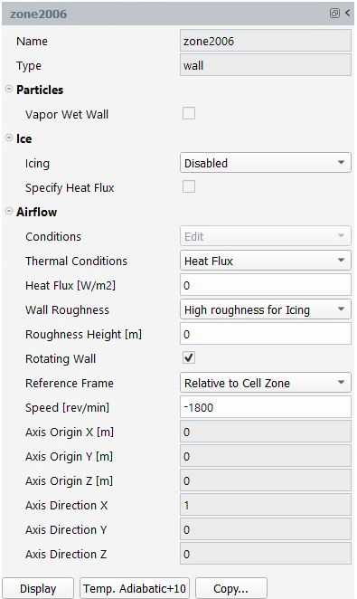
Note: Zone2006 corresponds to the shroud, which is not needed for icing computations and can be disabled. This is a static wall which does not rotate with the fan, and needs to be set as counter rotating to the cell zone. This is set by enabling and applying the opposite rotation speed. Alternatively you could set it to zero rotation in the absolute reference frame. The axis origin and direction will be locked to the same values used for the cell zone.
In the Particles section, retain the following setting:
Disable Vapor Wet Wall.
In the Ice section, retain the following setting:
for Icing.
In the Airflow section, retain the following settings:
for Thermal Conditions.
0for Heat Flux [W/m2].for Wall Roughness.
0for Roughness Height [m].Enable .
for Reference Frame.
-1800for Speed [rev/min]
Setup → Boundary
Conditions → Walls → zone2007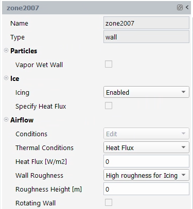
Note: The fan blade is zone2007. Icing will be enabled for this zone, with no additional rotational settings.
In the Particles section, retain the following setting:
Disable Vapor Wet Wall.
In the Ice section, retain the following setting:
for Icing.
In the Airflow section, retain the following settings:
for Thermal Conditions.
0for Heat Flux [W/m2].for Wall Roughness.
0for Roughness Height [m].Disable .
Setup → Boundary
Conditions → Walls → zone2008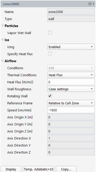
Note: The bypass/core splitter is zone2008 and is set as counter rotating since it's a static component similar to zone2006. Icing is also enabled for this zone to visualize the amount of ice that will accumulate on this boundary.
In the Particles section, retain the following setting:
Disable Vapor Wet Wall.
In the Ice section, retain the following setting:
for Icing.
In the Airflow section, retain the following settings:
for Thermal Conditions.
0for Heat Flux [W/m2].for Wall Roughness.
0for Roughness Height [m].Enable .
for Reference Frame.
-1800for Speed [rev/min]
Note: On counter rotating walls, the icing results will be circumferentially averaged akin to the mixing plane approach. This modeling approach accounts for many instances of blades rotating past this splitter section through the course of icing computed for a much longer period than the passage of a single blade across the periodic section.
Setup → Boundary
Conditions → Walls → zone2009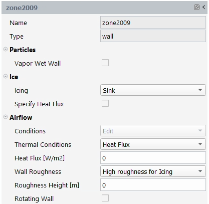
Note: Zone2009 is comprised of the trailing edge and the tip sections of the blade. Select this boundary, then press to show it in the Graphics window:
Note: The tip and the trailing edge have been separated on purpose to apply boundary conditions and prevent ice from accumulating on these parts. The mesh elements part of the structured grid are extremely thin with very high aspect ratios. This severely decreases the solver performance of the stress analysis module used for ice cracking. Water film flow requires extremely low time steps should there be any runback reaching these elements. The loss in ice-shedding modeling accuracy is negligible, while the gain in solver performance is quite significant. Therefore, it is highly recommended preparing your grids in a similar way for icing and ice shedding analysis on rotor blades.
In the Particles section, retain the following setting:
Disable Vapor Wet Wall.
In the Ice section, retain the following setting:
for Icing.
In the Airflow section, retain the following settings:
for Thermal Conditions.
0for Heat Flux [W/m2].for Wall Roughness.
0for Roughness Height [m].Disable .
Setup → Boundary
Conditions → Outlets → zone3010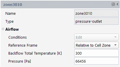
In the Airflow section, retain the following settings:
for Reference Frame.
300for Backflow Total Temperature [K].66456for Pressure [Pa].
Reset Conditions to .
Note: The Reference Frame is not used for outlet boundary conditions, therefore it can remain as . The only other options currently available are Backflow Total Temperature, in cases of flow reversal, and Pressure [Pa]. In rotating flows, there will be a radial pressure increase in the fluid due to centrifugal forces. The increase in pressure counters the centrifugal force on the fluid (radial equilibrium). In engine aerodynamic simulations, it is important to include this effect in the modeling process. Since this option is not present in Fluent Icing at this time, it will have to be set in the Fluent Solution workspace instead.
Setup → Boundary
Conditions → Outlets
zone3010 → Open the Fluent Workspace.
Project
→ Workspaces → Solution
A dialog will open advising you that the Fluent Solution Workspace will appear in another window. Press to proceed.
Set the Boundary Conditions of the simulation.
Setup → Boundary
Conditions →
Outlet → zone3010
(pressure-outlet, id=10)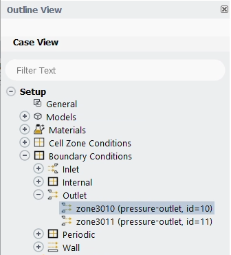
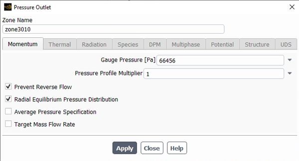
In the Momentum section, retain the following settings:
66456for Gauge Pressure [Pa].1for Pressure Profile Multiplier.Enable .
Enable .
Press to close this window.
Note: Apply the same settings for zone3011 (pressure-outlet, id=11).
Periodicity has already been set in the case, with one-to-one matching periodic boundaries with a 10-degree angle. Refer to Setting Up Periodic Boundaries for more information on setting periodicity for your domains.
Set the Solution properties of the simulation.
Solution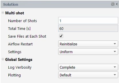
In the Multi-Shot section, retain the following settings:
1for Number of Shots.Enable .
for Airflow Restart.
for Settings.
In the Global Settings section, retain the following settings:
for Log Verbosity.
for Plotting.
Solution → Airflow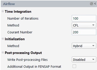
In the Time Integration section, retain the following settings:
100for Number of Iterations.Select under the Method drop-down list.
200for Courant Number.
Note: Time Scale Factor is a case specific setting and may need to be reduced for stability or increased for computational efficiency.
In the Initialization section:
Select under the Method drop-down list.
In the Post-processing Output section:
Retain the default selection of for Write Post-processing Files.
Solution → Particles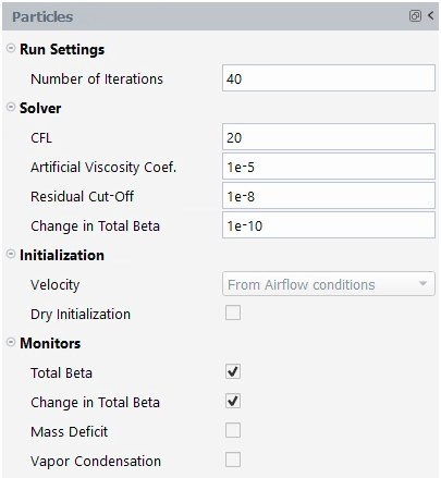
In the Run Settings section, retain the following setting:
40for Number of Iterations.
In the Solver section, retain the following settings:
20for CFL.1e-5for Artificial Viscosity Coef.1e-8for Residual Cut-Off.1e-10for Change in Total Beta.
In the Initialization section, retain the following settings:
The Velocity settings will be set to . The settings imported under the Airflow panel will be used.
Disable .
In the Monitors section, retain the following settings:
Enable .
Enable .
Disable .
Disable .
Note: This is a relatively simple case and 40 iterations will suffice to reach convergence. For more complex flows and meshes with thinner elements, the Number of Iterations should be increased. The best indicator in deciding whether your turbomachinery problem has converged lies is the . Collection efficiency will converge before total mass balance since the shadow zones may not have completely formed. It is important to converge the exit boundaries as well since in multi-row turbo simulations these exit rows will dictate the inflow conditions for subsequent rows.
Solution → Ice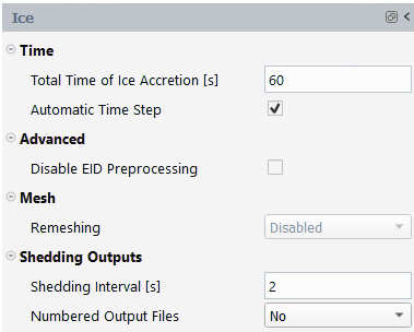
In the Time section, retain the following setting:
60for Total Time of Ice Accretion [s].Enable Automatic Time Step.
In the Shedding Outputs section, retain the following settings:
2for Shedding Interval [s].Note: The Shedding Interval [s] sets the frequency of ice stress and crack propagation analysis. Since this is a relatively expensive operation, it should not be set at every local time step. You can experiment with smaller and larger time intervals to explore how it affects the overall ice shedding properties like maximum shed-ice mass and the frequency of large shed events.
for Numbered Output Files.
Save the current simulation state.
Project
→ Simulation →
Launch the simulation.
Solution → Airflow → CalculateA New run window will appear. Set the Name of the new run to
flow.Once
flowis complete, follow the steps below. Solution → Particles → CalculateA New run window will appear. Set the Name of the new run to
particles.Once
particlesis complete, follow the steps below. Solution → Ice → CalculateA New run window will appear. Set the Name of the new run to
ice.Once the computation is complete, the solution files will be written inside the new run directory:
fan
flow
particles
ice
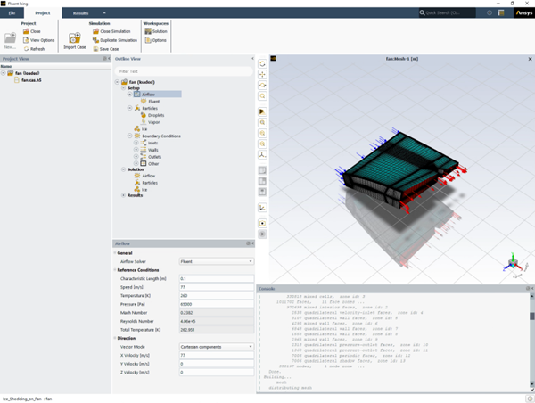
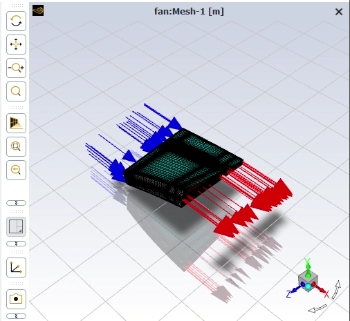
Take a look at the convergence history of this simulation in the Plots window located at the right of your screen.
The following three figures show the convergence of residuals of the Airflow, Particles and Ice runs.
Note: You can navigate to Results within the Outline View to display contour plots. Static pressure and temperature plots are already included under Contours.
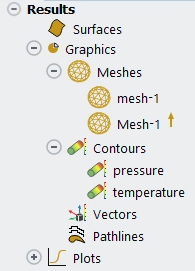
You can create a new contour plot to visualize the droplet solution in the window.
Results
→ Quick-View →
Contour → You can also open the results in Viewmerical from the . Right-click the Droplets solution and select → . A Viewmerical window will appear allowing you to further post-process the Droplets results.
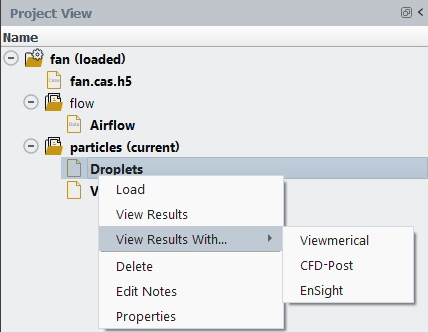
The image above shows the total ice mass history, and includes the ice accreting on the spinner as well. The drops in value indicate some ice loss due to shedding. The largest shed event occurs at t = 32s. The mass loss can be determined by clicking the curve at the two ends of the discontinuity and comparing the values of ice mass:
More information is available in a log file, fan.iceshed.log, located in the run directory on disk.
The Ice shedding summary log file shows 9 ice fragments were shed, with the total shed mass close to 50% of the total before shedding.
You can view the ice accumulation history as a sequence of results by right-clicking Ice under ice (current) in the Project View and selecting → to load the ice solution. Select if asked to append this solution to an existing Viewmerical window.
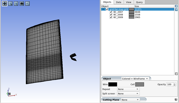
Using the – and + buttons in the top right corner, first remove this grid by clicking –, then click + to load a new dataset.
Under Grid file, click the browse button
 , navigate to the ice directory, and select
fan.ice.grid.shed.00000001. Enable the
option. For
Solution file (optional), click the browse
button and select fan.swimsol.shed.00000001.
When a numbered solution file similar to this is chosen, enable the
additional option that
appears.
, navigate to the ice directory, and select
fan.ice.grid.shed.00000001. Enable the
option. For
Solution file (optional), click the browse
button and select fan.swimsol.shed.00000001.
When a numbered solution file similar to this is chosen, enable the
additional option that
appears.
Press . You should now see the ice solution with Mass Caught displayed. Switch to the Data tab on the right panel and select from its drop-down. Set the Color range to and set the maximum range to
0.3.By moving the slider bar back and forth, you will be able to visualize the ice accumulation and mass loss due to shedding. The numbered files are saved at every 2 seconds of icing, coinciding with the shedding analysis frequency.
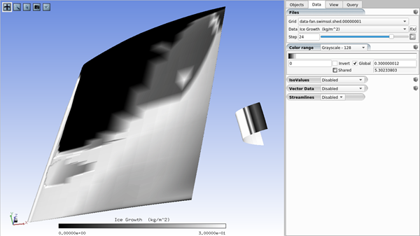
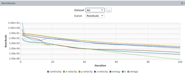
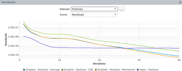
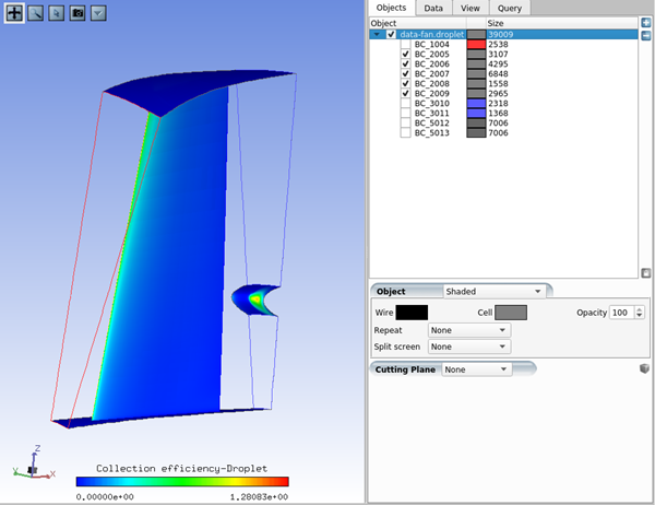
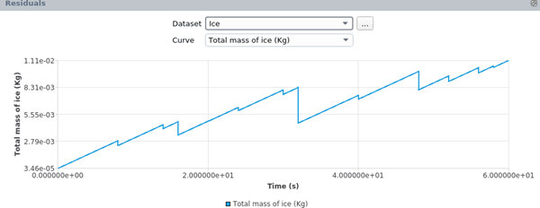
The following sections of this tutorial are:
For a list of limitations related to multi-shot, see Known Limitations in Fluent Icing 2024 R2.
This tutorial is divided into the following sections:
This tutorial demonstrates Fluent Icing's capabilities in conducting a multi-shot ice accretion simulation on the 3D Onera M6 swept wing under glaze icing conditions using automatic remeshing with Fluent Meshing. Automatic remeshing will maintain and/or improve the mesh resolution over the ice shape as it evolves at each shot. Therefore, it will enhance convergence, precision and accuracy of the entire simulation process.
Through this tutorial, you will learn how Fluent Icing can be set up to perform an 18-minute multi-shot ice accretion calculation divided into 6 quasi-steady shots of 3 minutes each. The automatic remeshing approach uses Fluent Meshing to entirely remesh the new iced surface as well as the volumetric mesh. It maintains a high level of mesh quality and precisely captures complex features such as ice horns.
Note: The automatic remeshing approach shown is different than the automatic mesh displacement (ALE) method. In the ALE method, only the ice surface and cells around the ice shape are displaced. This method maintains the same number of nodes and cells during the entire multi-shot simulation. The disadvantage of the ALE method is the deterioration of the mesh quality (coarsening, increase in aspect ratio of cells, etc.). This is especially true for longer ice accretion times where the possibility of complex ice shapes such as horns can develop.
You should have at least 64GB of RAM to run this multi-shot icing simulation since the mesh size increases with the number of shots.
Multishot Icing with Automatic Remeshing - Run in Batch Mode shows how to run a multi-shot icing simulation in Fluent Icing using batch mode and a journal file.
The problem considers the multishot ice accretion on the 3D Onera M6 swept wing under glaze icing conditions using automatic remeshing with Fluent Meshing.
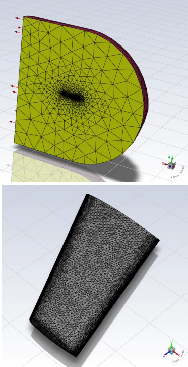
Table 1.1: Simulation In-Flight Icing Conditions
| Characteristic Length | 0.65 m |
| Speed | 103 m/s |
| Angle of Attack | 4° |
| Pressure (Altitude = 5000 ft) | 84312.727 Pa |
| Temperature | 268 K (-5.15 °C) |
| MVD | 20 μm |
| LWC | Appendix C - Continuous Maximum |
| Ice Accretion Time | 18 minutes |
The following sections describe the setup and solution steps for this tutorial:
To prepare for running this tutorial:
Download the
fluent_multishot.zipfile here .Unzip
fluent_multishot.zipto your working directory.The file, oneram6-wing.cas.h5, can be found in the folder.
Use the Fluent Launcher to start Ansys Fluent.
In the Fluent Launcher, set the Capability Level to Enterprise, then select Icing.
Set Solver Processes between
2and4.Click Start.
Alternatively, Fluent Icing can be opened using the icing (on Linux) or icing.bat (on Windows) file inside the fluent/bin/ folder.
Uncheck , , and .
Project
→ Workspaces →
Options
Create a new project file.
File → New
Project...Enter
Fluent_Icing_ONERAM6_Multishotas the Project file name within the Select File dialog.Select and import the oneram6-wing.cas.h5 input grid.
Project
→ Simulation → Import
Case
A New Simulation window will appear. Enter the Name of the New Simulation as
oneram6_icing, and check to enable . Click .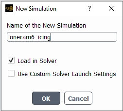
A new simulation folder will be created in the Project View, and the oneram6-wing.cas.h5 file will be imported.
After the .cas.h5 file has been successfully loaded, a new Outline View tree appears under oneram6_icing (loaded).
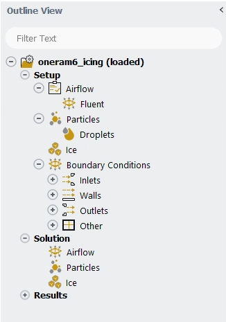
The mesh is now displayed in the Graphics window to the right.
Define the Simulation Type.
Setup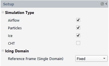
The , and Simulation Type should automatically be enabled within the Setup panel.
Set the Airflow properties for the simulation.
Setup → Airflow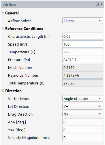
In the General section:
Retain the default selection of for Airflow Solver.
In the Reference Conditions section, retain the following settings:
0.65for Characteristic Length [m].103for Speed [m/s].268for Temperature [K].84312.7for Pressure [Pa].
In the Direction section, retain the following settings:
for Vector Mode.
for Lift Direction.
for Drag Direction.
4for AoA [deg.].0for Yaw [deg.].103for Vector Magnitude [m/s].
Set the Fluent properties for the simulation.
Setup →
Airflow → Fluent
Set to Default Air
PropertiesA dialog will open. Click to accept the air properties computed from the current airflow temperature.
Note: This automatically sets the air properties, suggested for icing simulations, from the current reference air temperature. The values of air properties have been computed using the equations presented in Airflow.
For simplicity, thermal conductivity and viscosity equations are shown below.


where
refers to the ambient air static temperature,
and , and are equal to 0.00216176
W/m/K3/2, 288 K and
17.9*10-6 Pa.s,
respectively.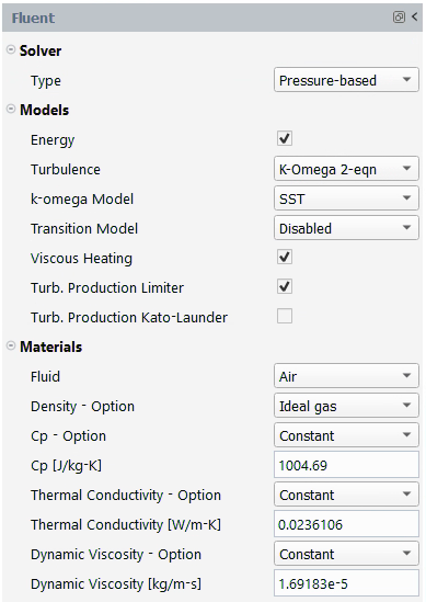
In the Solver section:
Retain the default selection of for Type.
In the Models section, retain the following settings:
Enable .
for Turbulence.
for k-omega Model.
for Transition Model.
Enable both Viscous Heating and Turb. Production Limiter.
In the Materials section, retain the following settings:
Select under the Fluid drop-down list.
for Density - Option.
for Cp - Option.
1004.69for Cp [J/kg-K].for Thermal Conductivity - Option.
0.0236106for Thermal Conductivity [W/m-K].for Dynamic Viscosity - Option.
1.69183e-5for Dynamic Viscosity [kg/m-s].
Open the Fluent Workspace.
Project
→ Workspaces → Solution
A dialog will open advising you that the Fluent Solution Workspace will appear in another window. Press to proceed.
Define the Viscous Model.
Setup →
Models → Viscous (SST
k-omega)In the Model Constants section, retain the following settings:
0.9for Energy Prandtl Number.0.9for Wall Prandtl Number.
Press to close this window.
Define the Reference Values.
Setup →
Reference Values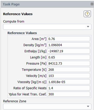
In the Reference Values section:
Set Area [m2] to
0.76.
Define the Report Definitions.
Solution →
Report Definitions
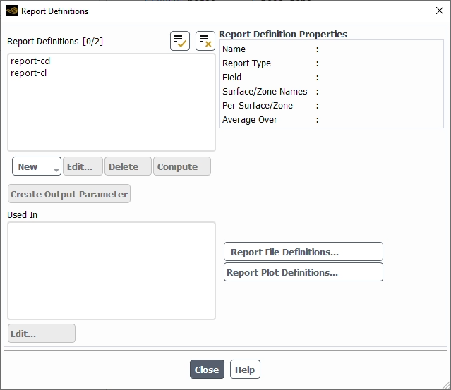
In the Report Definitions section:
Select report-cd and press (To create a new drag report, you can select → → )
Retain the default values of
0.99756405,0.069756474, and0for X, Y, and Z for Force Vector.Familiarize yourself with the selections in the Drag Report Definition dialog. Press to close this window.
De-select report-cd, select report-cl, and press (To create a new lift report, you can select → → )
Retain the default values of
-0.069756474,0.99756405, and0for X, Y, and Z for Force Vector.Familiarize yourself with the selections in the Lift Report Definition dialog. Press to close this window.
Press to close the Report Definitions dialog.
Modify the Absolute Criteria for convergence.
Solution → Monitors → Residual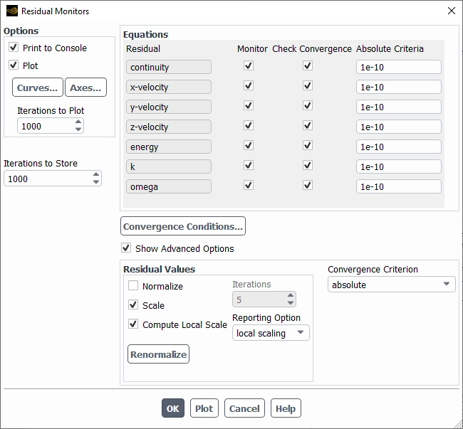
In the Equations section, retain the following settings:
Set
1e-10for all Absolute Criteria entries.and .
Enable .
Enable and .
Set for Report Option.
Press to close this window.
Maximize the Fluent Icing graphical user interface and close the Fluent Workspace.
Project
→ Workspaces → Solution
Set the Particles properties for the simulation.
Setup → Particles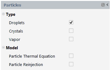
Enable under Type in the Particles panel.
Set the Droplets properties for the simulation.
Setup → Particles → Droplets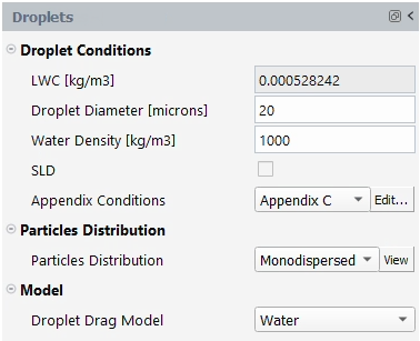
In the Droplet Conditions section, retain the following settings:
20for Droplet Diameter [microns].1000for Water Density [kg/m3].Select under the Appendix Conditions drop-down list and press .
Toggle on Continuous maximum (Stratiform clouds) in the Appendix C - Atmospheric Icing Conditions dialog and press .
The LWC [kg/m3] field automatically updates its value based on the previous selection.
In the Particles Distribution section:
Retain the default selection of for Particles Distribution.
In the Model section:
Retain the default selection of for Droplet Drag Model.
Set the Ice properties for the simulation.
Setup → Ice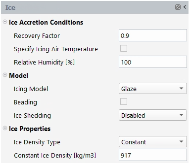
In the Ice Accretion Conditions section, retain the following settings:
0.9for Recovery Factor.100for Relative Humidity [%].
In the Model section:
Retain the default selection of for Icing Model.
In the Ice Properties section, retain the following settings:
for Ice Density Type.
917for Constant Ice Density [kg/m3].
Set the Boundary Conditions for your simulation.
Setup → Boundary
Conditions → Inlets → pressure-far-field-4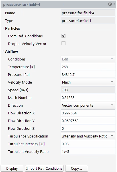
In the Airflow section:
Press on to import the reference conditions of the case file. All reference conditions are now imported to your boundary condition.
Retain all default selections under the Airflow section.
Note: will apply the droplet conditions at the inlet of the pressure-far-field boundary, which in this case is the LWC and MVD. If remains unchecked, the airflow velocity is imposed as the droplet velocity at the inlet. Therefore, the relative velocity between air and droplets is zero at farfield.
Setup → Boundary
Conditions → Walls → wall-5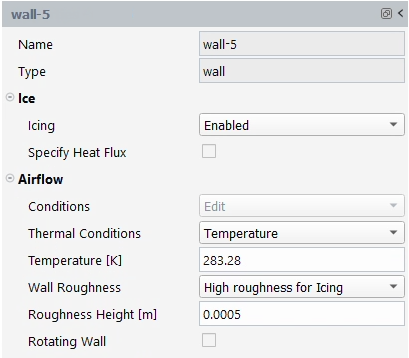
In the Airflow section, retain the following settings:
for Thermal Conditions.
Click to enter
283.28for Temperature [K].Select under the Wall Roughness drop-down list.
Set Roughness Height [m] to
0.0005.Note: This is the initial roughness height applied to the first shot only. All other shots will have a roughness distribution applied over their iced surfaces since was enabled under
Setup → IceRepeat the steps above for wall-6 and wall-7.
Setup → Boundary
Conditions → pressure-outlet-8
In the Airflow section:
Select under the Reference Frame drop-down list.
Press on to import the reference conditions of the case file. All reference conditions are now imported to your boundary condition.
Retain all default selections under the Airflow section.
Set the Solution properties of your simulation.
Solution → Airflow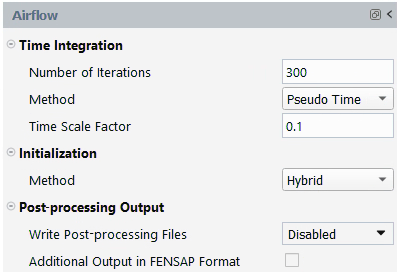
In the Time Integration section, retain the following settings:
300for Number of Iterations.Select under the Method drop-down list.
0.1for Time Scale Factor.
Note: Time Scale Factor is a case specific setting and may need to be reduced for stability or increased for computational efficiency.
In the Initialization section:
Select under the Method drop-down list.
In the Post-processing Output section:
Retain the default selection of for Write Post-processing Files.
Solution → Particles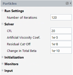
Retain all default selections under the Particles panel.
Solution → Ice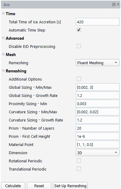
In the Time section:
Retain the default value of
180for Total Time of Ice Accretion [s].Press on to gain access to all Remeshing options.
In the Mesh section:
Retain the default selection of for Remeshing.
In the Remeshing section, retain the following settings:
[0.002, 3]for Global Sizing - Min/Max.1.2for Global Sizing - Growth Rate.0.003for Proximity Sizing - Min.[0.002, 0.02]for Curvature Sizing - Min/Max.1.2for Curvature Sizing - Growth Rate.20for Prism - Number of Layers.1e-6for Prism - First Cell Height.[1, 1, 0.05]for Material Point.for Dimension.
Note:
Large grids/meshes with small mesh sizing may run into memory problems at the solver to meshing switch.
A remesh_run.jou file is automatically created in the simulation folder. This file contains the automatic remeshing steps used by Fluent Meshing to create a new mesh at each shot. For advanced users of Fluent Meshing who have specific needs, you can modify this script as needed, by going to the Project View tab, right-clicking it and selecting . This provides more flexibility and allows you to adapt the journal file to your specific needs.
Launch the simulation.
Solution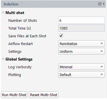
In the Multi-shot section, retain the following settings:
6for Number of Shots.Enable .
for Airflow Restart.
for Settings.
In the Global Settings section, retain the following settings:
for Log Verbosity.
for Plotting.
Note: The airflow solver can be reinitialized at each shot or continued from an interpolated solution originating from a previous shot. This can be done by either or under . For this tutorial, leave it to .
Launch the simulation by pressing .
A New run window will appear. Set the Name of the new run to
multishot_remeshingand press .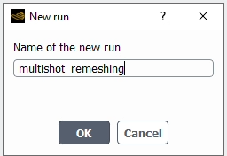
Note: Alternatively, you can launch the multi-shot calculation using
Solution Run
Multi-Shot
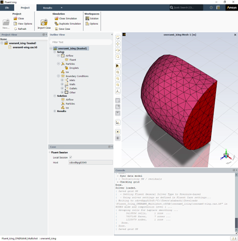
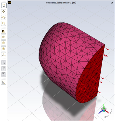
View your convergence history for all shots.
Project
View → multishot_remeshing View
ConvergenceYou can look at the convergence history of this simulation in the Curve → window located to the right of your screen. Dataset → , , provide a quick overview of the convergence history of all shots.
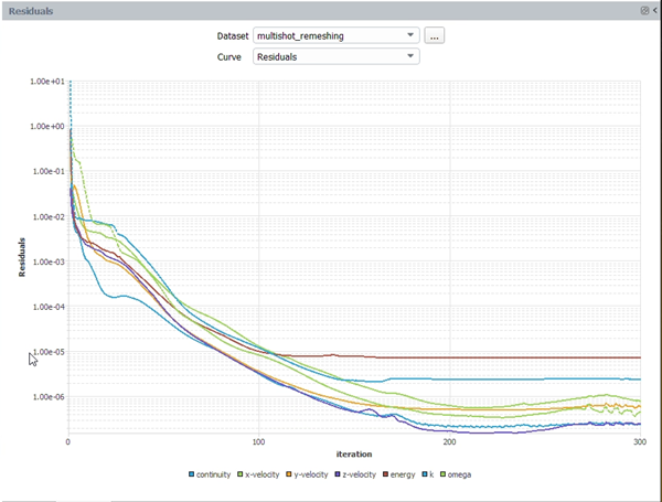
If your calculation stopped during the multishot simulation, you can resume it from a specific step within a shot. Go to the Project View, right-click the shot.xx folder, and select . Next, go to
Solution.
Inside its Solution panel, set the
Step from where you would like to resume your
multi-shot simulation, ,
, , and
. Then, click to relaunch your calculations. Click
to continue the current run. 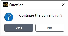
Calculations will start at the beginning of the step that was selected.
If you would like to restart your calculations with new settings, click followed by to reload the initial grid and reset all solutions. Make changes to your multishot calculation inside the Outline View and click .
Do not close Fluent Icing if you would like to further post-process the multi-shot ice solution.
Post-process your icing solution.
Project → Project
View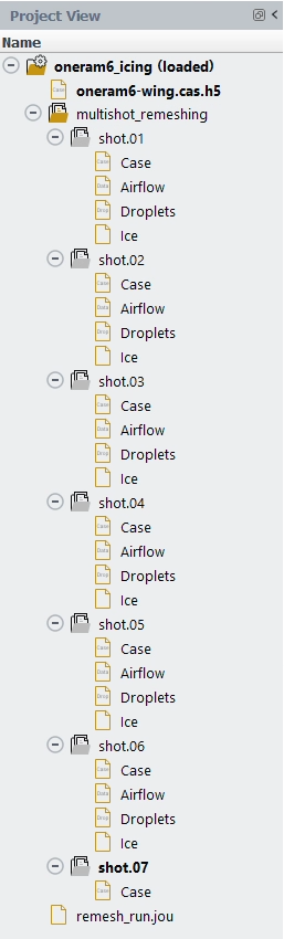
Under the oneram6_icing (loaded) simulation, a new run named multishot_remeshing now appears. Expand the run by clicking the + icon to the left of multishot_remeshing to show the files associated with the run. Each shot is represented by a folder and includes a two digit number to specify the shot number. Each folder contains a mesh file (Case), and 3 solution files (Airflow, Droplets and Ice).
Once all calculations are complete, you can view the final ice shape by right-clicking Ice located under shot.06 within the Project View. Select → . Choose in the View Ice dialog.
Note: You are also invited to perform another icing simulation with the following finer mesh settings. These settings will allow you to obtain a smooth representation of the ice shape but will require more computing resources.
Within
Solution → Ice,
modify the following settings under
Remeshing.Set Global Sizing - Min/Max to
0.001.Set Curvature Sizing - Min/Max to
0.001.Set Prism - Number of Layers to
25.
The figure below shows the ice shape obtained with these new conservative settings. These settings do a better job of capturing ice horns as well as the convective and viscous effects around the ice shape.
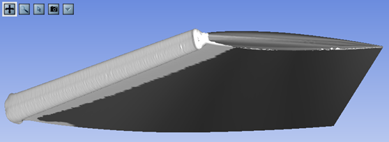
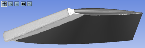
In this section, you will learn how to launch your icing simulation in Fluent Icing batch mode.
A python script that recorded all steps of the previous tutorial is used to demonstrate this capability.
Note: The python script was generated following these steps:
Open Fluent Icing
Select → . In the Select File window, name your script
oneram6-multishots-auto-run.py. Click to start the recording.Repeat all the steps of the previous tutorial and wait until the simulation is completed.
→ to finish the recording.
Open the script. Add the following few extra command lines at the beginning of the script if you want to delete an old existing project. In this case, the old project name is Fluent_multishot_oneram6:
Project.erase('Fluent_multishot_oneram6')preferences.PrjApp.UseLauncher.setState(False)preferences.PrjApp.ShowFluentWindow.setState(False)When running in batch mode, turn off the graphical user interface Launcher and the Fluent client.
Create a new working folder and name it
FLUENT-ICING.Download the
fluent_multishot.zipfile here . Extract all the files and copy oneram6-wing.cas.h5 and oneram6-multishots-auto-run.py to the working folder ../FLUENT-ICING/.Open a terminal and navigate to the working folder ../FLUENT-ICING/. Execute the following command to launch the run in batch mode within Fluent Icing on a Windows™ machine.
..\fluent\bin\icing.bat -R oneram6-multishots-auto-run.py -t 12
                            -N
To launch the run in batch mode on Linux machines, execute the following command:
../fluent/bin/icing -R oneram6-multishots-auto-run.py -t 12
                            -N
Replace the
..with the full path where the Ansys package is installed. The option-Rin the command means that Fluent Icing will execute the python scriptoneram6-multishots-auto-run.pythen exit. The option of-t 12is the number of CPU assigned to this run, 12 CPUs in this case. Use the-Noption to set Fluent Icing in batch mode. See Python Console for more details and available options.Once the script is executed, it will automatically create a project name/folder, set up the icing simulation, and launch the run. Fluent Icing will run in batch mode until the simulation completes.
Note: You can also run the script to set up the icing simulation without launching the simulation. To do so,
Open the script with any text editor.
Go to the end of the script, and comment out the last line to skip the execution step of the command by adding
#at the beginning of the line.# Project.newRun('multishot','multishot_remeshing',-1)Save and close the script.
Execute the script as mentioned in Step 3 above.
Launch Fluent Icing and go to → , or select Open... under the Project ribbon. Navigate to the working folder ../FLUENT-ICING, and select the file Fluent_multishot_oneram6.flprj to add the project to Fluent Icing’s Project Library.
Note: Fluent Icing will not automatically add new projects to its Project Library that are run in batch mode. The new project can be accessed by using → .
After the project is added, you will see it within the Project View:
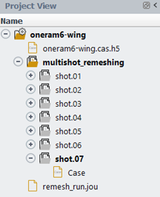
Verify that the results below are similar to those obtained in Multishot Glaze Ice with Automatic Remeshing Using Fluent Meshing by following the steps below:
Right-click multishot_remeshing under Project View and select to view the simulation’s convergence. The figures below show the 1st shot Residuals of the airflow simulations.
Figure 1.74: Residuals of 1st Shot’s Air Flow Simulation (Left: Script Run; Right: Simulation from the Multishot Icing with Automatic Remeshing on the Onera M6 Wing Tutorial)
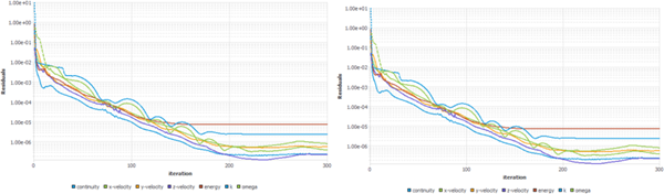
Right-click Ice under the shot.01 folder under Project View. Select → , and then click from the View Ice dialog. The following shows the ice surface solution of the 1st shot.
Figure 1.75: Instant. Ice Growth of 1st Shot Surface Icing Solution (Red: Script Run; Black: Simulation from the Multishot Icing with Automatic Remeshing on the Onera M6 Wing Tutorial)
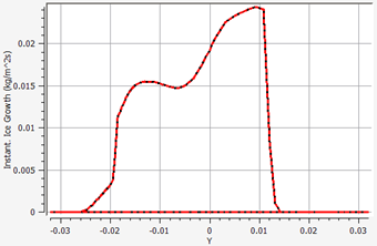
Figure 1.76: Water Film of 1st Shot Surface Icing Solution (Red: Script Run; Black: Simulation from the Multishot Icing with Automatic Remeshing on the Onera M6 Wing Tutorial)
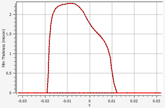
Figure 1.77: Wall Temperature of 1st Shot Surface Icing Solution (Red: Script Run; Black: Simulation from the Multishot Icing with Automatic Remeshing on the Onera M6 Wing Tutorial)
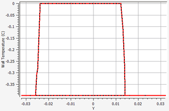
To view the final ice shape, right-click the Ice icon located under shot.6 in the Project View. Select → . Choose from the Information window to load the ice shape in a new Viewmerical window if you didn’t close the previous one. You will then choose in the View Ice dialog.
Figure 1.78: Computed Ice Shape at the End of the 6th Shot (Left: Script Run; Right: Simulation from the Multishot Icing with Automatic Remeshing on the Onera M6 Wing Tutorial)
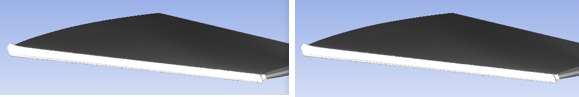
You can now post-process these icing results with CFD-Post. Consult the next section for more information.
In this tutorial, you will learn how to postprocess and generate figures and animations of a 3D Multishot ice accretion calculation (ice shape and ice solution fields) using two dedicated CFD-Post macros: Ice Cover – 3D-View and Ice Cover – 2D-Plot. For this purpose, the Multishot icing solutions of the multishot_remeshing run are needed and, therefore, completion of Multishot Glaze Ice with Automatic Remeshing Using Fluent Meshing is required.
For more information regarding these macros, consult the CFD-Post Macros section within the FENSAP-ICE User Manual.
In your Fluent Icing window, go to the Project View and right-click multishot_remeshing. Select .
A dialog will open asking you to select the type of dataset. Press on . A secondary window will then open asking you to select the type of Ice dataset. Press on .
After opening CFD-Post, a Domain Selector window will request confirmation to load the following domains: ice swimsol, map grid, and map swimsol. Click to proceed.

Go to the Calculators tab and double-click on Macro Calculator. The Macro Calculator’s interface panel will be activated and displayed.
Note: The Macro Calculator can also be accessed by selecting → from the CFD-Post’s main menu.
Select the macro script from the Macro drop-down list. This will bring up the user interface which contains all input parameters required to view ICE3D output solutions in the CFD-Post 3D Viewer.
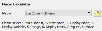
The default settings inside the Macro Calculator panel will allow you to automatically output the ice shape of a first shot of the Multishot simulation. Output the ice shape at the end of the multi-shot simulation of Multishot Glaze Ice with Automatic Remeshing Using Fluent Meshing, this corresponds to the ice shape of shot 6. Set Multi-shot # to
6.Under Display Mode, enter
0.2in Transparency to output a semi-transparent ice shape that will allow you to see the swept wing beneath the ice shape.Leave the other settings unchanged. Click to execute the macro and view the ice shape in 3D Viewer.
Note: To change the style of the ice shape display, go to Display Mode and select one of the following options: , , , or . To output the surface mesh of the ice shape, go to Display Mesh and select .
To output the solution fields of your icing simulation, you can either select , or under Display Mode. In this case, you will output the ice accretion rate over the ice layer without transparency.
To do this, select in Display Mode.
Set a Transparency value of
0under Display Mode as this will provide a more solid view on the displayed surfaces.Select in the Display Variable drop-down list.
You will change the range and number of contours of the ice solution field. Under Display Variable,
Set Number of Contours to
21.Change Range from to .
Enter
0.03and0in the (Usr. Specif.) Max and (Usr. Specif.) Min input boxes, respectively.
Click to view the instantaneous ice growth over the final ice shape.
Go to Save Figure to save this figure in a file,
Select beside Save Figure.
Keep Screen Shot under By. If you select Size, you must specify width and height of the image.
Keep the default Format. There are three types of format supported: , , and . The default format is .
Specify a Filename for the figure.
Click to generate and save the figure. A message will appear to notify the user of the location where the figure is saved.
Note: If CFD-Post was opened through Fluent Icing, the figure will be saved in the run folder. If CFD-Post was opened in standalone mode, the figure will be saved in the Window’s system default folder.
You can also generate and save animations that highlight the ice shape evolution of your Multishot simulation while displaying an ice solution field over it. Follow these steps to create and save a custom animation.
Go to Save Figure and select .
Go to Multi-shot # and set it to
1. The animation starts at the assigned shot number in Multi-shot # to the last shot of the simulation.Set (Multi-shot) Movie to and click to see the animation on the 3D Viewer window.
To save this animation, in (Multi-shot) Movie,
Set Save to .
Keep the default Format. Two formats are supported, and . The default is .
Specify a Filename.
Click to generate and save the animation. A message will appear to notify the user of the location where the animation is saved and at which shot the animation starts.
Note: If CFD-Post was opened through Fluent Icing, the animation will be saved in the run folder. If CFD-Post was opened in standalone mode, the animation will be saved in the Window’s system default folder.
Select from the Macro drop-down list to create 2D-plots of the Multishot simulation. You will create 2D-Plots at various locations along the swept wing using a single shot solution or multiple shot solutions.
Set Multi-shot # to
3since you will output the ice shape of the third shot.Change the Plot’s Title to
Multishot – Remeshing – Shot No.3.Keep the default setting of 2D-Plot (with). The default setting is . The other options of 2D-Plot (with) allow the creation of multiple shot results within the same 2D-Plot.
Under 2D-Plot (with),
Keep the default setting of Mode. The default setting is Geometry to output the ice shape.
Make sure Cutting Plane By is set to the default Z Plane.
Set X/Y/Z Plane Point to
0.5. In this case, this corresponds to a Z=0.5 plane.Set the X-Axis to and the Y-Axis to .
To center the 2D-Plot around the wing section at Z=0,
Keep the (x)Range of the X-Axis to Global.
Change the (y)Range of the Y-Axis from Global to User Specified. Specify values of
0.15and-0.15in the input boxes of (Usr.Specif.y)Max and (Usr.Specif.y)Min, respectively.
Leave the other default settings unchanged and click to create a 2D-Plot of the 3rd shot ice shape at Z=0.5 in ChartViewer. Adjust the output window’s size. The figure below shows the cutting plane location in the 3D Viewer window and the output of the macro in ChartViewer.
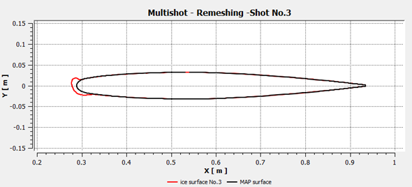
You will now create a 2D-Plot of all the ice shapes of the multishot simulation using a user-defined cutting plane and save this image in a file. First, set Multi-shot # to
1.Change the Plot’s Title to
Multishot – Remeshing – All Shots.Select from the 2D-Plot (with) drop-down list. This will generate a series of 2D plot curves, starting from the assigned shot number in Multishot Num. to the last shot of the multishot simulation.
Under 2D-Plot (with),
Keep the default setting of Mode. The default setting is Geometry to output the ice shape.
Set the Cutting Plane By to Point and Normal to define an arbitrary cutting plane. The normal does not need to be a unit vector.
Set the coordinate of the point (
0.533646,-0.022681,0.898708) inside (Pt. & Nml.)Pnt.X/Y/Z, respectively.Set the normal vector coordinates (
0.5,0,0.866025) inside (Pt. & Nml.)Nml.X/Y/Z, respectively.Set the X-Axis to X and the Y-Axis to Y.
To center the 2D-Plot around the leading edge of the wing section defined by the arbitrary cutting plane,
Change the (x)Range of the X-Axis from Global to User Specified. Specify values of
0.65and0.45in the input boxes of (Usr.Specif.x)Max and (Usr.Specif.x)Min, respectively.Change the (y)Range of the Y-Axis from Global to User Specified. Specify values of and in the input boxes of and , respectively.
To simultaneously save this 2D-Plot as a figure, go to ,
Select beside Save Figure.
Keep the default Format. There are three types of format supported: , , and . The default format is .
Specify a Filename for the figure.
Leave the other default settings unchanged and click to create a 2D-Plot of all the ice shapes at a user-defined cutting plane in ChartViewer. A message will appear to notify the user of the location where the figure is saved. Adjust the output window’s size. The figure below shows the cutting plane location in the 3D Viewer window and the output of the macro in ChartViewer.
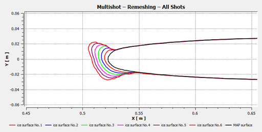
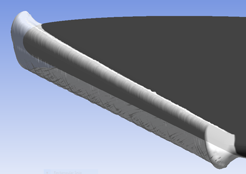
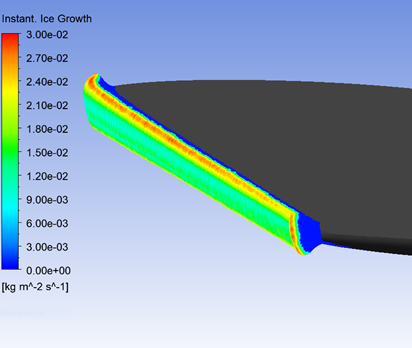
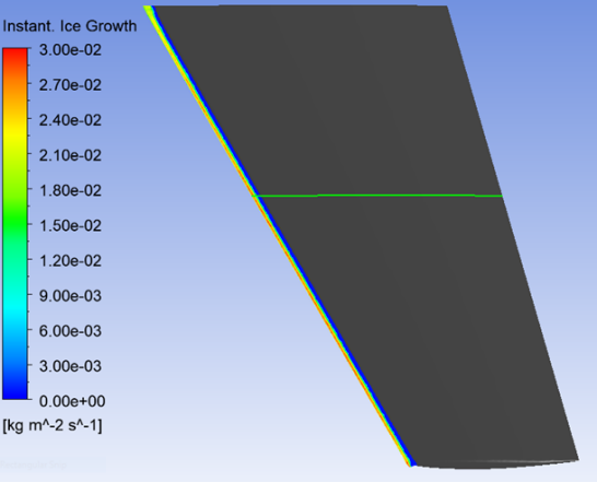
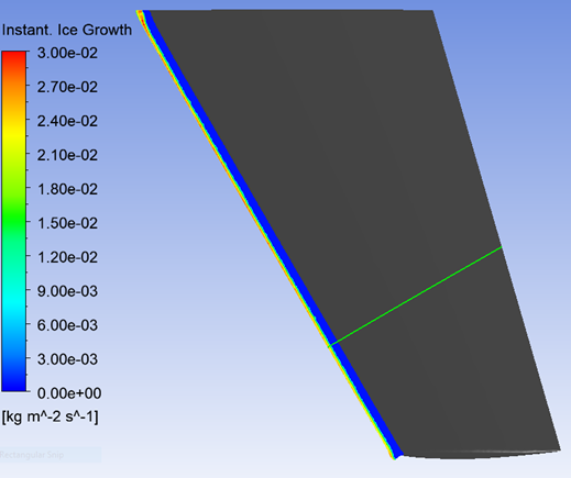
This chapter introduces Fluent Icing's Conjugate Heat transfer for anti-icing simulation. Anti-icing systems are vital for assuring aircraft safety and performance, especially in inclement weather where ice accumulation on critical surfaces such as wings, engine inlets, and sensors can compromise aerodynamic performance and represent a safety risk. These systems often use heated surfaces, pneumatic boots, or chemical de-icing to prevent or remove ice. This chapter provides a step-by-step lesson on a hot-air piccolo tube anti-icing system on an aircraft wing.
The physics and thermodynamics of in-flight icing involve:
Strong heat convection in fluids
Heat conduction through solids
Droplet impingement
Surface water film flow
Water evaporation
Change of phase
Ice formation
Conjugate Heat Transfer (CHT) refers to the thermal transfer between fluid and solid domains. Anti-Icing CHT is a steady-state simulation in which a heat balance on the target surfaces is achieved at the end of convergence. This steady-state solution denotes the equilibrium condition in which the heat input from the anti-icing system equals the heat loss due to convective cooling and ice formation.
Fluent Icing's anti-icing CHT simulation includes the following steps:
Fluent CHT in dry air condition
Particle impingement
Initial water film and ice accretion
Wet air anti-icing
In Fluent, the dry air simulation can be configured in the same way as conventional intrinsic CHT. This step should be done in Fluent rather than Fluent Icingg. To test the convergence of CHT computation, proper heat transfer monitors can be established at fluid-solid interfaces. Once the dry air CHT has fully converged and the solution has been confirmed, it can be imported into Fluent Icing for the next steps. Wet air CHT computation requires particle impingement, an initial water film, and ice accretion. During the initial Ice run, an extra step called EID will be performed internally to extract surface convective heat transfer coefficients. You will then be able to evaluate the heat transfer coefficients and ensure that they are within the acceptable range.
This tutorial is divided into the following sections:
This tutorial demonstrates how to simulate a hot air anti-icing system inside the leading edge of a wing using Fluent Icing CHT. The metal skin at the leading edge separates the cold wet air that flows over the external skin surface from the hot internal airflow. Hot air jet are discharged from the orifice of the piccolo tube heating the metal skin of the leading edge to prevent ice accretion on the external surface.
It is highly recommended that you study the relevant sections in Modeling Conductive and Convective Heat Transfer in the Fluent User's Guide prior to working on this tutorial.
As an input to Fluent Icing CHT, an intrinsic Fluent CHT setup in dry air conditions should be configured and prepared. It is highly recommended to run dry air conditions before wet air computations as it is easier to adjust Fluent settings before moving on to Fluent Icing. In this tutorial, grids are separated for the external, internal, and solid domains. Follow Piccolo Tube Anti-Icing in Wet Air Using Fluent in the Ansys FENSAP-ICE Tutorial Guide for more information regarding the boundary conditions and the material qualities employed in this case.
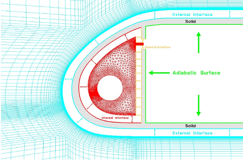
The following sections describe the setup and solution steps for this tutorial:
To prepare for running this tutorial:
Download the fluent_icing_cht.zip file here .
Unzip fluent_icing_cht.zip to your working directory.
The file, FLUENT-piccolo-ext.cas.h5, can be found in the folder.
Launch Fluent 2024 R2 on your computer.
Within the Fluent Launcher, select Solution.
Set Solver Processes to
8or more under Parallel (Local Machine).Click Start.
Load the external flow case file.
File → Read
→ Case...Select FLUENT-piccolo-ext.cas.h5 as the Case File within the Select File dialog and press .
Append the internal flow file FLUENT-piccolo-int.cas.h5.
Domain
→ Zones
→ Append → Append Case
File...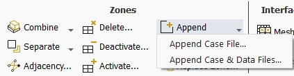
A Warning dialog will appear regarding zone id changes due to the case file being appended. Click to close this dialog.
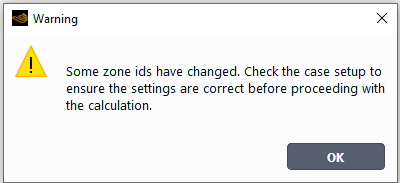
Next, append the solid case file FLUENT-piccolo-solid.cas.h5. Fluid, solid cell zones and their corresponding materials are now available in the Outline View.
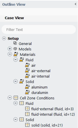
Note: Model parameters such as operating pressure, boundary conditions and material properties are already set in the .cas.h5 files as they are part of Piccolo Tube Anti-Icing in Wet Air Using Fluent in the Ansys FENSAP-ICE Tutorial Guide. You can review these settings to learn more about the simulation conditions.
Create the mesh interfaces between fluid and solid domains.
Setup → The thermal conditions will be exchanged between the three domains via non-conformal mesh connections formed by pairing the overlapping wall boundaries. Fluent can automatically select a pairing from a list of wall zones. The interfacing boundary zone names are prefixed with cht- to facilitate this selection process. There are no constraints on what can be used as a prefix, and there is no necessity to use one. It is recommended that you use a similar naming strategy so that you can easily identify interfaced borders in your own simulations. Industrial scale simulations will almost certainly contain dozens of boundary zones where a naming approach like this can be useful.
Select all fluid-solid interface boundaries from the Wall list of Boundary Zones using the prefix cht- and click Create. Fluent will automatically pair and generate mesh interfaces. There are three Mesh Interfaces in this example:
intf:01:cht-1-solid::cht-1-ext - Interface between external fluid and solid.
intf:02:cht-2-solid::cht-2-int - First interface between internal fluid and solid.
intf:03:cht-3-solid::cht-3-int - Second interface between internal fluid and solid.
The Console displays the percentage of matching area from both sides of the mesh interface. A decent mesh interface pair will show an exact or almost 100% area percentage.
Press to proceed to the next step.
Note: If the original grid contains conformal coupled walls between fluid and solid domains, it is required to slit them into uncoupled walls first, then create non-conformal interfaces for Fluent Icing CHT simulation. This additional step can be done in Fluent console with TUI command:
/mesh/modify-zones/slit-face-zone.Update the Reference Values.
Physics → Reference
Values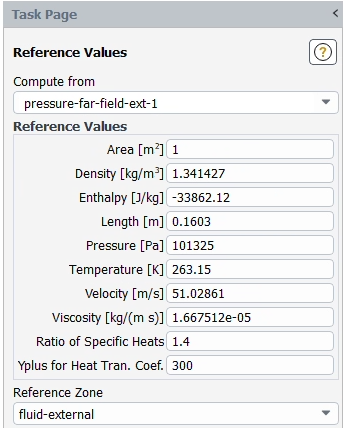
In the Reference Values section, retain the following settings:
for Compute from.
1for Area [m2].1.341427for Density [kg/m3].-33862.12for Enthalpy [J/kg].0.1603for Length [m].101325for Pressure [Pa].263.15for Temperature [K].51.02861for Velocity [m/s].1.667512e-05for Viscosity [kg/(m s)].1.4for Ratio of Specific Heats.300for Yplus for Heat Tran. Coef.for Reference Zone.
Specify the Solution Methods.
Solution → Methods
Select under Pseudo Time Method.
Note: The CFL method can also be used for the air flow calculations and could lead to better convergence, depending on the case. When you apply this CHT setup on a different case, study both time integration methods to find out which leads to better and more stable convergence. You should look at the convergence of total heat flux monitors on boundaries of interest to gauge the performance of either method.
Although it is advised that gradients be used in aero computations, gradients are employed in this case to avoid some oscillations in heat flow at the wall/symmetry plane intersection.
Create a new Flux Report at the CHT interfaces.
Solution → →
→ 
In the Flux Report Definition dialog, retain the following settings:
total-heat-transfer-ratefor Name.intf:01:cht-1-solid::cht-1-ext-shadow for Boundaries.
Note: This boundary will experience droplet impingement and runback water film outside of the wall surface while also experiencing strong conductive heating through solid metal. The heat exchange in this case becomes very intense. Therefore, it is more important to monitor this interface rather than others. The total heat transfer rate at the interface will be used to verify the convergence of CHT calculation. You are also encouraged to create your own reports that cater to your own simulation.
Retain all other default values and settings and press .
Initialize the solution.
Solution → → 
Select under Initialization Methods.
Click to change Number of Iterations to
20.
Set your Run Parameters.
Solution → 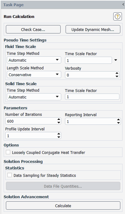
In the Solid Time Scale section, retain the following setting:
1for Time Scale FactorNote: Time Scale Factor can remain at 1 for the fastest rate of convergence but may need to be reduced as low as
0.01for some cases that have a difficult time converging the air flow.
In the Parameters section, retain the following setting:
600for Number of Iterations.
Launch the run by clicking .
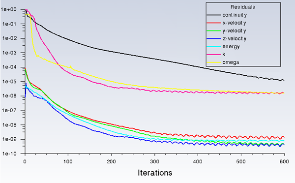
Important: Verify the dry air solution before moving onto the wet air simulation. If needed, make any adjustments and re-calculate the solution until you are satisfied with the results.
Save your solution.
File
→ Write → Case &
Data...Save and name both case and data files as
piccolo-dry-airand close Fluent.
Creating a Fluent Icing Project and Simulation
After validating results calculated in Fluent, the .cas/.dat files can both be imported into Fluent Icing for calculating wet air conditions.
Use the Fluent Launcher to start Ansys Fluent.
In the Fluent Launcher, set the Capability Level to Enterprise, then select Icing.
Set Parallel Processing Options to
8.Click Start.
Alternatively, Fluent Icing can be opened using the icing (on Linux) or icing.bat (on Windows) file inside the fluent/bin/ folder.
Uncheck , , and .
Project
→ Workspaces →
Options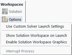
Create a new project file.
File → New
Project... Enter
piccolo-wet-airas the Project file name within the Select File dialog.Select and import the piccolo-dry-air.cas.h5 input grid saved in the previous steps.
Project
→ Simulation → Import
Case.A New Simulation window will appear. Enter the Name of the New Simulation as
piccolo-wet-air-cht, and check to enable . Click .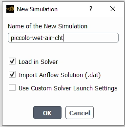
A new simulation folder will be created in the Project View, and the piccolo-dry-air.cas.h5 file will be imported.
After the .cas.h5 file has been successfully loaded, a new Outline View tree appears under piccolo-wet-air-cht (loaded).
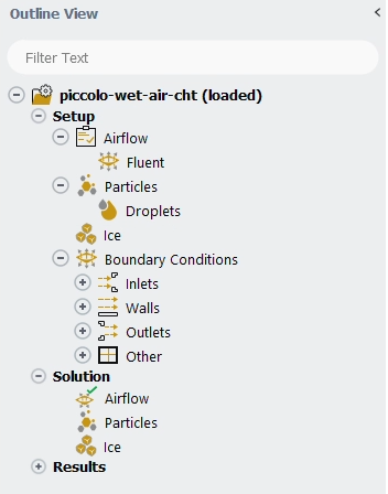
The mesh is now displayed in the Graphics window to the right.
Define the Simulation Type.
Setup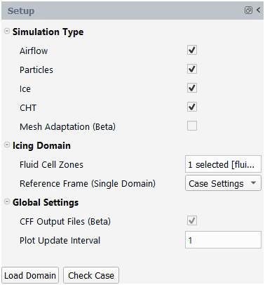
In the Simulation Type section, retain the following setting:
Enable , , and under Simulation Type.
In the Icing Domain section, retain the following setting:
fluid-external for Fluid Cell Zones.
Note: Particle impingement and water film calculations are computed on the external domain only.
for Reference Frame (Single Domain).
Click to load the icing domain into the icing solver. Save your case.
Project
→ Simulation → Save
Case Note: Only after pressing can the solver identify the icing domain. A window will appear informing you that the current grid has a changed topology. Icing computations will be performed on the chosen subdomain. Click . It's also a good idea to save the case after choosing an icing domain so that this information is saved in the Fluent case file.
Set the Airflow properties of the simulation.
Setup → Airflow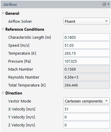
In the General section, retain the following setting:
for Airflow Solver.
In the Reference Conditions section, retain the following settings:
0.1603for Characteristic Length [m].51for Speed [m/s].263.15for Temperature [K].101325for Pressure [Pa].
In the Direction section, retain the following settings:
for Vector Mode.
51for X Velocity [m/s].0for Y Velocity [m/s].0for Z Velocity [m/s].
Set the Fluent properties of the simulation.
Setup → Fluent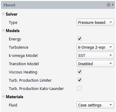
In the Solver section, retain the following setting:
for Type.
In the Models section, retain the following settings:
Enable Energy.
for Turbulence.
for k-omega Model.
Enable Viscous Heating.
Enable Turb. Production Limiter.
In the Materials section, retain the following setting:
for Fluid.
Set the Particles properties of the simulation.
Setup → Particles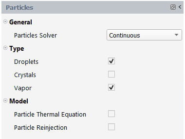
In the General section, retain the following settings:
for Particles Solver.
In the Type section, retain the following settings:
Enable and .
Note: It is highly recommended to enable vapor for more accurate computation of local vapor pressure. Vapor pressure is critical to evaporative heat flux calculation, which is an important term in water film transport equations.
Set the Droplets properties of the simulation.
Setup → Particles → Droplets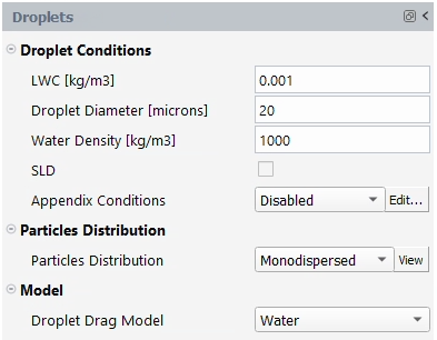
In the Droplet Conditions section, retain the following settings:
0.001for LWC [kg/m3].20for Droplet Diameter [microns].1000for Water Density [kg/m3].Disable .
for Appendix Conditions.
In the Particles Distribution section, retain the following setting:
for Particles Distribution.
In the Model section, retain the following setting:
for Droplet Drag Model.
Set the Vapor properties of the simulation.
Setup → Particles → Vapor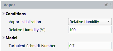
In the Conditions section, retain the following settings:
for Vapor Initialization.
100for Relative Humidity [%]
In the Model section, retain the following setting:
0.7for Turbulent Schmidt Number.
Set the Ice properties of the simulation.
Setup → Ice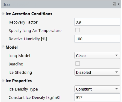
In the Ice Accretion Conditions section, retain the following settings:
0.9for Recovery Factor.Disable Specify Icing Air Temperature.
100for Relative Humidity.
In the Model section, retain the following settings:
for Icing Model.
Disable Beading.
In the Conditions section, retain the following settings:
for Ice Density Type.
917for Constant Ice Density [kg/m3].
Set the Boundary Conditions of the simulation.
Setup → Boundary
Conditions → InletsNote: The inlet boundary conditions are the same as the initial conditions. Therefore, no changes are required here.
Set the Solution properties of the simulation.
Solution → Particles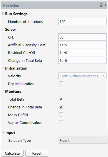
In the Run Settings section, retain the following setting:
120for Number of Iterations.
In the Solver section, retain the following settings:
50for CFL.1e-5for Artificial Viscosity Coef.1e-6for Residual Cut-Off.1e-6for Change in Total Beta.
In the Initialization section, retain the following settings:
The Velocity settings will be set to . The settings imported under the Airflow panel will be used.
Disable .
In the Monitors section, retain the following settings:
Enable .
Enable .
Disable .
Disable .
Solution → Ice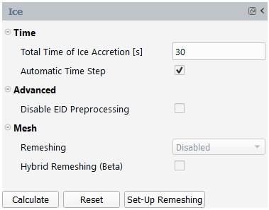
In the Time section, retain the following setting:
30for Total Time of Ice Accretion [s].Enable Automatic Time Step.
Note: The icing total time entered here is not the anti-icing CHT simulation total time. Anti-icing simulations are steady-state calculations that aim to achieve thermal equilibrium. Because ICE3D is a transient solver, it takes some time to build the water film distribution for each CHT iteration. The total icing duration entered here is intended to assist ICE3D in reaching a steady-state solution within each CHT iteration.
Launch the simulation.
Solution → Particles → CalculateA New run window will appear. Set the Name of the new run to
droplets-vapor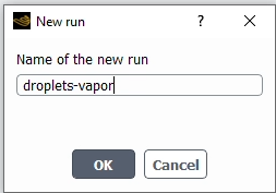
Once
droplets-vaporis complete, follow the steps below. Solution → Ice → CalculateA New run window will appear. Set the Name of the new run to
ice.
Once
iceis complete, follow the steps below. Solution → CHTNote: Before running CHT, ensure that the Airflow, Particles, and Ice have completed successfully.
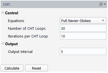
In the Control section, retain the following settings:
for Equations.
30for Number of CHT Loops.10for Iterations per CHT Loop.
In the Output section, retain the following setting:
5for Output Interval.
Solution → CHT → CalculateA New run window will appear. Set the Name of the new run to
cht-wet-air.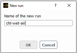
Once the computation is complete, the solution files will be written inside the new run directory:
piccolo-wet-air-cht
droplet-vapor
ice
cht-wet-air
Verify droplet and vapor solutions within Viewmerical
Project
View → droplet-vapor → Droplets → You can also use Viewmerical to view the ice cover.
Project
View → ice → Ice → When prompted, click to view the ice solution on the walls.
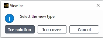
The convergence of the CHT computation can be analyzed using convergence and monitor plots. The residual curves show periodic rise in the convergence history, which indicates the starting of each CHT loop. Once the CHT computation completes, the convergence curves gradually becomes flat. The total heat transfer rate, maximum and minimum temperature at CHT interfaces are all stabilized approaching the end of computation. From the Project View on the left of the panel, each saved intermediate solution is available and can be viewed by right-clicking the object.
View the final ice solution.
Project
View → cht-wet-air → loop.30 → Ice → Verify the film thickness, instantaneous ice growth rate, and wall temperature. The anti-icing power has led to a running wet condition at the leading edge. Some ice residual is seen at the unprotected zone due to frozen of runback water.