The following sections of this chapter are:
- 7.1. Unsteady Heat Conduction with Phase Change
- 7.2. Piccolo Tube Operating in the Dry Air Regime
- 7.3. Piccolo Tube Operating in the Wet Air Regime (Anti-Icing)
- 7.4. Piccolo Tube Anti-Icing in Wet Air Using Fluent
- 7.5. Piccolo Tube Anti-Icing in Wet Air Using CFX
- 7.6. Unsteady Electro-Thermal De-icing in Wet Air
- 7.7. Unsteady Electro-Thermal De-icing in Wet Air Using Fluent with FENSAP-ICE
- 7.8. Electro-Thermal Simulation of a Heating Element
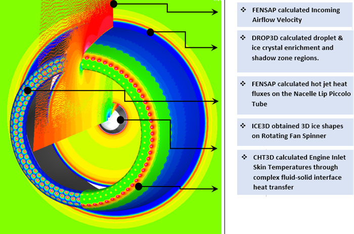
- 7.9. Axisymmetric Nacelle Anti-Icing System Operating in the Wet Air Regime – Droplets & Crystals
This 2D test-case is intended to demonstrate the operation of the electro-thermal de-icing equipment in the skin of an iced wing section. The geometry consists of a thin rectangular multi-layered solid with 5, 3.125 cm-wide heater pads (A, B, C, D, E), each having a power density of 32,000 W/m2. In this test-case, the thickness of the heating elements is neglected. The geometry is shown below:
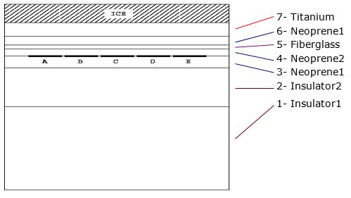
The innermost level of the solid (from bottom) is composed of two layers of different insulators, followed by two layers of neoprene, one layer of fiberglass, one layer of neoprene and finally, the outside layer of titanium. A uniform 1.9 mm-thick ice layer has accumulated at the top. The lateral edges and the inside boundaries are insulated, while the outside boundary is exposed to convection, with a constant heat transfer coefficient of 450 W/m2/K. The initial temperature in the structure, as well as the surface recovery temperature, are both set to 266.15 K (-7 °C). The five elements are heated in a 10 second, D-E-C-B-A sequence with an idle time of 10 seconds at the end. The boundary condition indices of the heater pads are:
| Heater | BC Index |
|---|---|
| A | 6061 |
| B | 6062 |
| C | 6063 |
| D | 6064 |
| E | 6065 |
Create a new project using → or the New project icon. Name this project
Heat.Create a new run using → or the new run icon. This tutorial uses C3D as the heat conduction solver. Choose an appropriate name for the run.
Download the
7_CHT3D_Advanced.zipfile here .Unzip
7_CHT3D_Advanced.zipto your working directory.Double-click the grid icon to assign a grid file. Select the grid file 2D_5HEAT_ICE_SMALL.grid provided in the tutorials subdirectory ../workshop_input_files/Input_Grid/C3D.
The grid is a hexa mesh with 4,130 elements and 8,520 nodes. The grid file contains the grid coordinates, the element connectivity table, the material index and the table of boundary surfaces (8,568 faces including the 5 heater pads).
Double-click the config icon to assign the input parameters for C3D.
Go to the Settings panel. In the Initial conditions section, set the value of Temperature to
266.15K (-7 °C).Go to the Properties panel. Add new materials and their physical properties by clicking on the button. In this particular test case, seven different materials should be created: Ice, Fiberglass, Insulator1, Insulator2, Neoprene1, Neoprene2, and Titanium.
For each material, the Density, Conductivity and Enthalpy should be defined.
For ice, the density Distribution should be constant and set to
917kg/m3. Since ice can melt and become water, set both its Thermal Conductivity and Enthalpy to Temperature dependent to simulate phase change. Set the Number of Temperature points to 6 for Thermal Conductivity, and use the following table of conductivity as a function of temperature:Table 7.1: Thermal Conductivity vs. Temperature for H2O
Temperature (K/C) Thermal Conductivity (W/(m K)) 243.15 K (-30 °C) 2.55 273.15 K (0 °C) 2.55 273.1501 K (0.0001 °C) 0.558 283.15 K (10 °C) 0.577 313.15 K (40 °C) 0.633 348.15 K (75 °C) 0.671 Set the Number of temperature points to
3for Enthalpy and use the following table of enthalpy as a function of temperature:Table 7.2: Enthalpy vs. Temperature for H2O
Temperature (K/C) Enthalpy (J/kg) 273.15 K (0 °C) 579849.6 273.1501 K (0.0001 °C) 944080.8 373.15 K (100 °C) 1399910.4 Table 7.3: Material Properties
Material Density (kg/m3) Thermal Conductivity (W/m/K) Enthalpy at 0°C (J/kg) Insulator 1 50 0.250 9375366.0 Insulator 2 89 0.250 5267059.5 Neoprene 1 160 0.293 8787187.5 Neoprene 2 160 0.293 4064813.0 Fiberglass 2700 0.313 393160.4 Titanium 4540 17.03 141310.5 Go to the Materials panel. Click the material Name (MAT_X) in the table at the top of the panel to display its corresponding grid volume in the Graphical window. In the Material Association section, link each volume ID present in the grid to a material using the Material type (defined in 7) pull-down menu:
MAT_1 → Insulator 1
MAT_2 → Insulator 2
MAT_3 → Neoprene 1
MAT_4 → Neoprene 2
MAT_5 → Fiberglass
MAT_6 → Neoprene 1
MAT_7 → Titanium
MAT_8 → Ice
Review the material properties one by one once they are all entered.
Go to the Boundaries panel. Set the boundary conditions as follows:
BC_2020 is the upper surface of the ice layer, which is subject to convection heat transfer. In the BC definition section, use the pull-down menu to select a Mixed boundary condition. Set the value of Temperature to
266.15K and Heat coefficient to450W/m2/K.BC_2021 groups all other external surfaces of the assembly, which are insulated. Select the Flux boundary condition with the pull-down menu and set the value of Heat flux to
0.BC_6061 to BC_6065 are the 5 heater pads. Click the boundary condition name to display the selected pad in the Graphical window. The Heat flux value for each heater should be kept as
0W/m2 in the BC definition sections. These are the baseline values for the heaters that would be constantly applied outside of defined cycles.
Go to the Cycles panel. The simulation consists of a sequence of six different BC Cycles, each lasting 10 seconds. To add a BC Cycle, click
 next to the Cycle drop-down menu. This will create
the first cycle A with some default settings. The green bar is the
“on” time of the selected heater in this cycle. By default it starts at the
beginning of the cycle and covers 100% of the cycle. You will use this style to define a
separate cycle for each heater, that are 10 seconds long each. For the first cycle
A set the Duration to
next to the Cycle drop-down menu. This will create
the first cycle A with some default settings. The green bar is the
“on” time of the selected heater in this cycle. By default it starts at the
beginning of the cycle and covers 100% of the cycle. You will use this style to define a
separate cycle for each heater, that are 10 seconds long each. For the first cycle
A set the Duration to 10seconds. Then choose Heater 61 from the BC menu in the Current selection section.All heaters in each cycle are turned off by default. Modify each cycle as follows:
Turn on Heater D (BC_6064) during Cycle #1
Turn on Heater E (BC_6065) during Cycle #2
Turn on Heater C (BC_6063) during Cycle #3
Turn on Heater B (BC_6062) during Cycle #4
Turn on Heater A (BC_6061) during Cycle #5
All heaters are turned off in Cycle #6 for an idle period of 10 seconds.
Set Heat Flux to Constant and at
32000W/m2.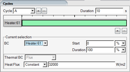
To add a new heater cycle, click
next to the Cycle menu again. A dialog will appear
prompting to copy or create a new empty cycle. Click Yes to copy
Cycle
A to Cycle
B.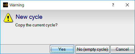
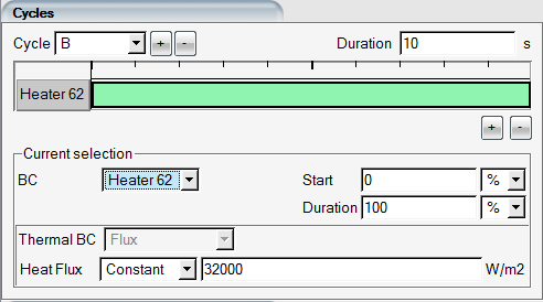
Change Heater 61 to Heater 62 in the BC drop-down menu to finish setting up this cycle for the 2nd heater.
Repeat copying of the cycles until all five heaters are defined as cycles A through E.
Finally, click
one last time to create cycle F as a new empty cycle.
Click the green bar that comes by default and click  at the bottom right corner of the green bar to remove it. This should make
this cycle an empty cycle:
at the bottom right corner of the green bar to remove it. This should make
this cycle an empty cycle: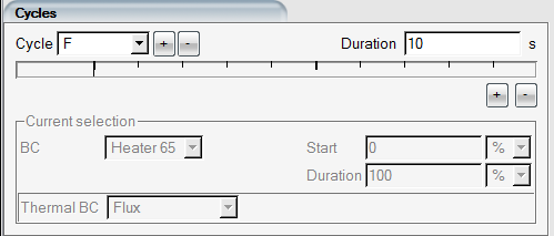
Now that all cycles are ready, queue them up in the Sequence box in the following order:
D,E,C,B,A,F(separated by commas).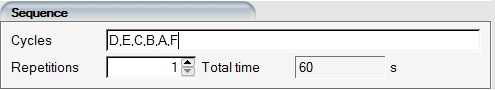
Select the Solver panel. Set the value of Time step to
0.1seconds and the Total time to60seconds (the five heater pads are each turned on and off sequentially for 10 seconds, followed by an idle period of 10 seconds).Set the value of Time period between printout to
10seconds.Run the calculation on
4CPUs if possible. The unsteady minimum and maximum temperatures are shown in the convergence window.To view the solution files saved at every 10 seconds, click the button and choose the file struc1.SOL.000001. This is the solution file output at time = 10s. Make sure that the default post-processor is Viewmerical. You will be asked if you would like to load the numbered data set:
For now, click , you will load each file separately. If you click yes, the numbered data files will be loaded as one set, and you will be able to cycle through them with a slider bar in the Data panel of Viewmerical.
Go back to the run window and click View again, this time choose struc1.000002 from the dropdown list. Append it to the Viewmerical window. Repeat the process for the remaining files 000003 through 000006.
At this point all six solutions should be loaded in Viewmerical. Go to Data panel and click the lock button. Switch to Query panel and enable the 2D plot.
In the 2D plot section, change the Target to Walls, Cutting plane to Y and the cut location to 0.0084. This is the interface between the titanium and the ice layer. Change the horizontal axis to X. All 6 temperature curves should be visible at this point. You can turn them on/off by clicking the data set names displayed just below the graph. You can use the Curve settings in the cube menu (top right) to change the colors and line weights. To easily change the graph window size, press Ctrl and double-click the 2D Plot menu title to detach the 2D graph from Viewmerical.
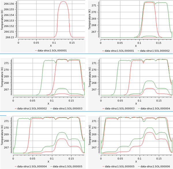
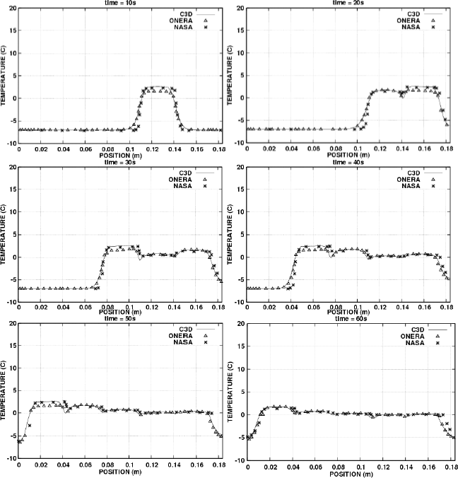
Figure 7.1: Temperature Profiles at the Ice/Titanium Interface, with ONERA, DRA, and NASA Codes Comparison
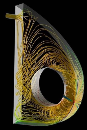
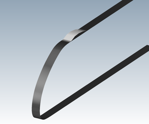
This tutorial illustrates the procedure to use CHT3D to compute the Conjugate Heat Transfer (CHT) through the metal skin of a leading edge, which separates the cold air flowing over the external skin surface from the hot internal air flow induced by the jet discharging from the orifice of the piccolo tube. In this first section, there are no droplets considered and the anti-icing system is said to be operating in dry conditions.
FENSAP-ICE’s approach to conjugate heat transfer consists of solving different domains separately, using a weak coupling technique. After converged steady-state solutions are obtained on the fluid domains, heat transfer across fluid/solid interfaces are iterated to convergence while the temperature in the solid and fluid domains are updated after each main CHT iteration. This modularized approach is very flexible, allowing different flow solvers to be used in the CHT algorithm. It also permits setting different reference, initial, and solver settings for the different domains which makes the convergence process more robust. The third advantage is the smaller size of individual grid and solution files for each domain, which makes post processing simpler.
The tutorial proceeds in three steps:
Computing the external cold air flow.
Computing the internal hot air flow.
Conjugate heat transfer across the domains through the solid metal skin.
Create a new project using → menu or the New project icon and name it
PICCOLO. Select the Metric units system.Create a FENSAP run in this project using the → menu or the new run icon and name it
FENSAP_ext.Double-click the grid icon and select the grid file grid_ext provided in the tutorials subdirectory ../workshop_input_files/Input_Grid/CHT.
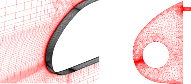
The mesh is a hexahedral grid with 234,960 nodes. The grid file contains the grid coordinates, the element connectivity table and the table of boundary surfaces.
Double-click the config icon to proceed to the input parameters setup.
Go to the Model panel. Select the Navier-Stokes option for the Momentum equations and Full PDE for the Energy equation.
Select the Spalart-Allmaras option for the Turbulence model and set the Eddy/laminar viscosity ratio to
1e-5.In the Transition box, choose Free transition. In anti-icing simulations, since no ice (roughness) is expected, free transition should be used in external flows to capture the laminar flow regions more accurately. Otherwise, the heat transfer coefficients may be over predicted by the fully turbulent (no transition) mode.
Go to the Conditions panel. Set the Reference conditions as follows:
Characteristic length 0.1603mAir velocity 51.03m/sAir static pressure 101325PaAir static temperature 263.15K (-10°C)In the Initial solution section, select the Velocity components option and set the Velocity X component to
51.03m/s (same as the reference Air velocity). The other velocity components should be set to0m/s.Go to the Boundaries panel. Select the inlet boundary BC_1000 and choose the Subsonic option in the Type tab. Click the button to set the Inlet conditions.
Select the wall boundary BC_2001. Set Surface type to No-slip and set the Temperature value by right-clicking in the temperature box and Copy from… → Adiabatic stagnation temperature + 10.
Note: Temperature must be specified on the leading edge BC_2001 in order to compute an initial heat flux to start the CHT calculation. This temperature will subsequently be updated automatically during the CHT3D loop.
Repeat the same settings for the family BC_2002.
Select the outflow boundary BC_3000. Choose the type as Subsonic, and click the button to set the exit pressure value to Reference conditions.
Go to the Solver panel. Select the Steady option in the Time integration pull-down menu. Set the value of the CFL number to
200and the Maximum number of time steps to1,000. Uncheck the Use variable relaxation option.Choose the Streamline upwind option in the Artificial viscosity tab. Set the Cross-wind dissipation coefficient to
1.e-9and move the slider to100% Second order position.Go to the Out panel. Save the Solution every
50iterations in Overwrite mode.Click the button to switch to the execution window. Choose
4or more CPUs if possible and start the computations. The average residual of the flow should reach about 4e-9 by the end of the run.The calculations may take some time depending on the number of available CPUs. The converged solution is provided in the tutorials subdirectory ../workshop_input_files/Input_Grid/CHT/soln_ext if you do not wish to wait for the results before proceeding to the next tutorial.
Create a new FENSAP run and name it
FENSAP_int.Double-click the grid icon to assign the grid file. Select the grid file grid_int provided in the tutorials subdirectory CHT. The mesh is a hybrid unstructured grid with 222,369 nodes.
Double-click the config icon to open the FENSAP input parameters window.
Go to the Model panel. Select the Navier-Stokes option for the Momentum equations (viscous flow) and Full PDE for the Energy equation.
Select K-omega SST as the Turbulence model and set the Eddy/laminar viscosity ratio of
1.e-5and the Turbulence intensity to0.0008.Go to the Conditions panel and set the following Reference conditions:
Characteristic length 0.05mAir velocity 367.2557m/sAir static pressure 101325PaAir static temperature 335.4K (62.25°C)The Characteristic length setting has no impact on the flow, but it will change the scale of the average residual which is reported in non-dimensional form. A large characteristic length will make the average residual appear smaller. It is a good practice to choose a characteristic length that matches the scale of the computational domain. In this case, 0.05m is the diameter of the piccolo tube.
In the Initial solution section, select the Velocity components option. Set the three components of velocity to
0m/s. Initializing internal cavities like the piccolo chamber with 0 velocity is recommended.Go to the Boundaries panel. Select the inlet family BC_1000. In the Type tab, select the Supersonic or far-field option from the pull-down menu and set the following conditions:
Pressure 101502.4PaTemperature 335.4K (62.25°C)Velocity X -345.107471232m/sVelocity Y -125.608847151m/sVelocity Z 0m/sThese conditions specify an orifice velocity with a Mach number slightly above 1. The velocity vector is perpendicular to the inlet surface and its orientation corresponds to an Angle of attack of -160 degrees. The vector can be displayed in the Graphics window by clicking the small cube icon at the right of the BC Inlet parameters tab.
Set the wall boundary conditions as follows:
BC_2002 No-slip Temperature 320K (46.85°C)BC_2003 No-slip Heat flux 0w/m2BC_2004 No-slip Temperature 320K (46.85°C)Note: Temperature must be specified on the interfacing boundary condition families to initiate the heat transfer between the two domains (air and solid). In this case BC_2002 will be interfacing with the leading edge part of the solid, and BC_2004 will interface with the back plate. These temperatures will be updated automatically during the CHT3D loop, as conduction takes place in the solid.
Select the BC_3000 family and click the button in the Type tab. Set the Pressure value to
101325Pa. This is the exit pressure opening to the external free stream flow.Go to the Solver panel. Select the Steady option in the Time integration pull-down menu. Set the value of the CFL number to
300and the Maximum number of time steps to1000. Click the Use variable relaxation check box and keep default values of Time steps and Relaxation factor. In the Advanced solver settings panel, reduce the Convergence level to1e-12, so that FENSAP does not stop prematurely.Note: This CFL number is a bit large but works well with the provided grid which is rather simple. For more complex configurations and larger pressure ratios, lower CFL numbers may be necessary for convergence. There is usually an optimum CFL number for each grid and conditions, which takes the solution to convergence fastest. Low CFL values will take longer to converge, while very high values can result in some unwanted oscillations in the transient solution (beginning of the iteration process) that will take additional time to clear out. This case for example runs with a high CFL number and takes many iterations to converge heat fluxes. Since the CFL number used is high, you should lower the convergence criteria, so that FENSAP does not stop prematurely.
Choose the Streamline upwind option in the Artificial viscosity tab. Set the Cross-wind dissipation coefficient to
1.e-9and move the slider to100% Second order position.Go to the Out panel. Save the Solution every
50iterations in Overwrite mode.Click the button to switch to the execution window. Use
4or more CPUs if possible.This calculation may take a long time to complete depending on the number of CPUs available. The converged solution is provided in the tutorials subdirectory ../workshop_input_files/Input_Grid/CHT/soln_int. If you do not want to wait for the run to finish, you can use this file to begin the next tutorial.
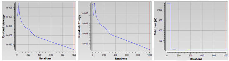
The two main convergence indicators for this run are the average residual and the total heat flux. The average residual and the energy equation converge to 1e-10 in approximately 700 iterations. However, changes in total heat are still visible. The run should be allowed to continue until the total heat flux converges well. The total heat flux curve should reach an asymptotic value of about 59 Watts. You can zoom on convergence curves by holding Shift and left-click. Middle-click to undo the zoom.
This section illustrates the Conjugate Heat Transfer procedure (CHT3D) required to couple the external and internal flow calculations of Initial External Flow Calculation and Initial Internal Flow Calculation by considering the heat conduction through the solid wall interface in order to determine the equilibrium temperature distribution in the solid.
Note: CHT3D can couple structured and unstructured grids without any limitations.
Create a new CHT3D run and name it
CHT3D_dry. The CHT configuration window will appear to prompt for the type of CHT simulation desired. Select Piccolo (2 fluids, 1 solid) in the Problem type pull-down menu, then choose Dry air. Press the button to continue with the setup. A tree of coupled FENSAP and C3D runs will appear in the run window.Drag & drop the config icon of the FENSAP_ext run (Initial External Flow Calculation) onto the fluid_ext config icon in CHT3D_dry. This automatically links the external grid, the flow solution and heat fluxes computed in the FENSAP_ext run to the input of the CHT3D_dry fluid_ext run.
If the previous tutorials were allowed to run to convergence, then you can keep the soln and hflux.dat files to the left of the config icon unchanged. Otherwise, replace them with soln_ext and hflux_ext files found in the tutorials subdirectory ../workshop_input_files/Input_Grid/CHT. Simply double-click the icons to browse to this directory.
Double-click the fluid_ext config icon to set up the input parameters for the external flow domain.
Go to the Solver panel. Increase the CFL number to
20000and change the Maximum number of time steps to10iterations. In this simulation, you will only run the energy equation and keep the flow constant. This allows the usage of a very large CFL number.In the Advanced solver settings section, reduce the convergence criteria to
1e-12, so that FENSAP does not stop prematurely. At each CHT3D iteration, FENSAP will complete 10 iterations before exchanging boundary conditions with the solid domain. It is crucial that fluid domains perform several iterations of their own at each CHT step in order to apply the updated boundary conditions properly. Otherwise CHT iterations will converge very slowly.Close and save the configuration file of fluid_ext.
Drag & drop the config icon of the FENSAP_int run (Initial Internal Flow Calculation) onto the fluid_int run in CHT3D_dry. This automatically links the internal grid, the flow solution and heat fluxes computed in the FENSAP_int run to the input of fluid_int run.
Similar to 2, if the solution files of the FENSAP_int run are not fully converged, replace the icons to the left of the config icon of the internal run by soln_int and hflux_int found under tutorials subdirectory ../workshop_input_files/Input_Grid/CHT.
Double-click the config icon to edit the input parameters for the internal flow.
Go to the Solver panel. Increase the CFL number to
20000and change the Maximum number of time steps to10iterations. Disable the Use variable relaxation option.Reduce the convergence criterion to
1e-12in the Advanced solver settings section.Close and save the configuration file of fluid_int.
To begin setting up C3D for the solid heat conduction, double-click the grid icon in the solid run in CHT3D_dry. Select the file grid_solid provided in the tutorials subdirectory CHT.
Double-click the config icon of the solid heat conduction run to edit the heat conduction parameters.
Go to the Settings panel. Set the value of Temperature of
300K (26.85°C). This will be the initial temperature throughout the solid domain. It is a reasonable initial guess between the external and internal static air temperatures.Go to the Properties panel. Click the Rename button to change the material name from default to
duralumin. Then set the Distribution of all properties to Constant. Specify the following characteristics for the material:Density 2787kg/m3Conductivity 164W/m/KEnthalpy 241060J/kgGo to the Materials panel. Since duralumin is the only material in the solid domain, the label MAT_0 will be automatically assigned to it.
Go to the Boundaries panel. Define the boundary conditions of the outer surfaces of the solid as follows:
BC_2001: Default settings (Thermal BC definition set to Nothing)
BC_2002: Default settings (Thermal BC definition set to Nothing)
BC_2004: Default settings (Thermal BC definition set to Nothing)
BC_2005: Set Thermal BC definition to Type: Flux, and set Heat flux to
0W/m2/KBC_2006: Set Thermal BC definition to Type: Flux, and set Heat flux to
0W/m2/KBC_2007: Set Thermal BC definition to Type: Flux, and set Heat flux to
0W/m2/KBC_4100: Set Thermal BC definition to Type: Flux, and set Heat flux to
0W/m2/KBC_4300: Set Thermal BC definition to Type: Flux, and set Heat flux to
0W/m2/K
CHT3D will automatically update the boundary conditions on BC_2001, BC_2002, and BC_2004 during the simulation.
Go to the Solver panel. Set the Time step to Automatic. Set the Maximum time step value to
0.1seconds and the Total time to5seconds. At each CHT3D iteration, heat conduction will be updated every 5 seconds. Close and save the configuration.C3D total time per CHT3D iteration can be considered as the overall time step of the conjugate heat transfer problem. Reducing this value will improve the stability of CHT runs while increasing it may hinder convergence to steady state temperature distribution in the solid.
Double-click the main config icon of the CHT3D_dry to set up the links between the solid and fluid domains.
Go to the Parameters panel. Set the Number of CHT iterations to
30and Solution output every 0 iterations (default value).Choose the Solve energy only option in the Flow solver mode pull-down menu for both internal and external flows.
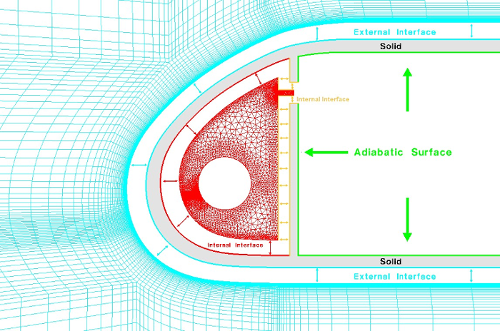
Go to the Interfaces panel. There are three fluid/solid interfaces in the computational domain. CHT3D will automatically exchange the boundary conditions between these three interfaces. Set up the interfaces as follows:
For External to Solid: There is only one interface between the external domain and the solid. Set the interface boundaries as follows:
External fluid grid: 2001
Solid grid: 2001
For Solid to Internal: There are two interfaces between the solid and the internal domain. Set the first interface as follows:
Solid grid: 2002
Internal fluid grid: 2002
Then click the
 button next to Interface label to add the third interface and set it as
follows:
button next to Interface label to add the third interface and set it as
follows:Solid grid: 2004
Internal fluid grid: 2004
Note: In this case, the interface boundary condition family numbers across the two grids are adjusted so that they match, which is not a requirement. The only requirement is that the interface boundary conditions overlap nicely, with no gaps and discontinuities. They do not have to be node-to-node matching.
Go to the Temperatures panel. Set the value of Recovery factor to
0.9.Right-mouse click the main config icon of CHT3D_dry, then select the option in the menu to launch the CHT3D calculation. Choose
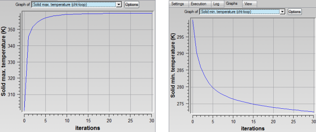
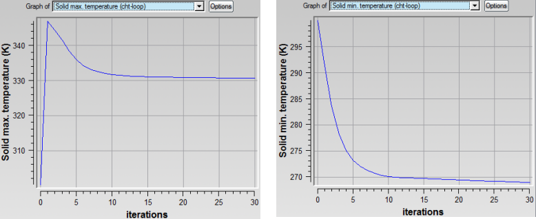
4CPUs in both the Execution settings and CHT settings section, if possible.Figure 7.11: CHT3D Solution: Convergence History of the Maximum (Left) and Minimum (Right) Solid Wall Temperature
Load the solid solution by clicking the button, and choosing Solid – Temperature from the drop-down menu.
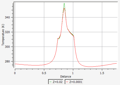
Figure 7.13: Temperature Distribution vs Wrap Distance on the External Surface of the Solid at Z = 0.0001 m and Z=0.02 m
Note: The automatic time stepping option in CHT3D improves the stability of the simulation. Under certain circumstances, this has the potential to decrease the total simulation time. However, if automatic time stepping substantially reduces the time step, this could result in an increase in total simulation time. In these situations, it may be beneficial to run with constant time stepping.
Create a new CHT3D run and name it
CHT3D_dry_constant_timestep. The CHT configuration window will appear to prompt for the type of CHT simulation desired. Select Piccolo (2 fluids, 1 solid) in the Problem type pull-down menu, then choose Dry air. Press the button to continue with the setup. A tree of coupled FENSAP and C3D runs will appear in the run window.Drag & drop the config icon of the CHT3D_dry run onto the CHT3D_dry_constant_timestep configuration. Select Full copy to copy all of the input files and configurations of each simulation component, including the main config, from the previously simulated CHT3D_dry run.
Double-click the config icon of the solid heat conduction run to edit the heat conduction parameters.
Go to the Solver panel. Set the Time step to Constant. Set the Time step value to
0.1seconds and the Total time to5seconds. Close and save the configuration.Right-mouse click the main config icon of CHT3D_dry, then select the option in the menu to launch the CHT3D calculation. Choose
4CPUs in both the Execution settings and CHT settings section, if possible.To compare the temperature solutions obtained with automatic time stepping to those obtained with constant time stepping, first load the first solid solution by right-clicking c3dsol of CHT_dry and choosing View with VIEWMERICAL. Next, right-click the c3dsol of CHT3D_dry_constant_timestep and choose View with VIEWMERICAL followed by Append. The two grids should be loaded with the temperature solutions showing. Split the screen to put the data sets on either sides of the view.
Figure 7.14: Temperature Contours on the Solid Surfaces Showing That the Auto Time Step Solution (Left) and the Constant Time Step Solution (Right) Provide Similar Results
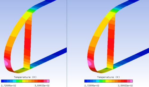
Figure 7.15: Temperature Distribution vs Wrap Distance on the External Surface of the Solid at Z = 0.0001 M Showing That the Auto Time Step Solution and the Constant Time Step Solution (the Curves Are Overlaid) Provide Similar Results
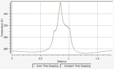
Note: In this simulation, the solid constant time stepping approach produced a similar solution to the solid automatic time stepping approach, and the simulation time was 3x faster. This may be the case in some situations, however, in other cases there may be stability problems or the simulation time may increase.
This tutorial illustrates the procedure to use CHT3D to compute the Conjugate Heat Transfer (CHT) through the metal skin of a leading edge, which separates the cold wet air flowing over the external skin surface from the hot internal air flow induced by the jet discharging from the orifice of the piccolo tube. A hot jet from the orifice of a piccolo tube heats the inner skin of the leading edge to prevent ice accretion on the outer surface. In this simulation FENSAP, DROP3D and ICE3D will be used to simulate the external flow conditions. C3D simulates the heat conduction through the solid leading edge skin and FENSAP will be used to simulate the internal flow.
To set up a CHT3D wet-air simulation, initial internal and external flow simulations are required, just as the dry air test case, with the addition of a water droplet and an initial ICE3D simulation.
This tutorial has the same flow conditions as Initial External Flow Calculation and Initial Internal Flow Calculation for both external and internal flow domains. Proceed with this tutorial if these sections were completed.
Create a new DROP3D run and name it
DROP3D_ext.Drag & drop the config icon of FENSAP_ext onto the config icon of the new DROP3D run. This copies the reference conditions of the flow to the droplet run.
Double-click the DROP3D_ext config icon to edit the parameters.
Go to the Conditions panel. Set the following Droplet reference conditions:
Liquid Water Content
1g/m3Droplet diameter
20micronsWater density
1000kg/m3
Go to the Boundaries panel. Select the BC_1000 (Inlet) boundary condition and click the Import reference conditions button.
Go to the Solver panel. Set the CFL number to
20and the Maximum number of time steps to300.Click the button. Start the calculation on
4or more CPUs if possible.
The goal of this step is not to provide an initial ice shape, but rather to establish a water film on the outer surface of the solid as an initial condition for the wet CHT3D run.
Create a new ICE3D run and name it
ICE3D_ext.Drag & drop the config icon of the DROP3D_ext (External Water Droplets Calculation) onto the config icon of this new run. This operation automatically links the air and droplet solutions, the grid of the external domain and the reference conditions to the ICE3D_ext run.
Double-click the config icon to edit the input parameters.
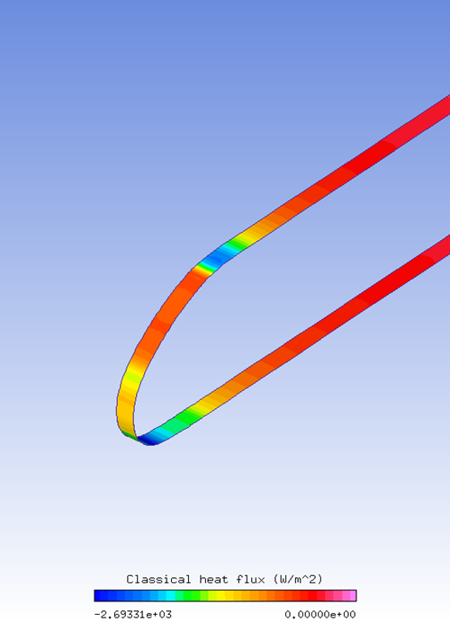
Go to the Model panel. Icing model should remain as Glaze - Advanced. Change the heat flux type to Classical.
In the Conditions panel set the Recovery factor to
0.9. The remaining settings were automatically transferred from the DROP3D configuration.Go to the Solver panel. Keep the Automatic time step option enabled and change the total time of ice accretion to
30seconds.Run the calculation on
4or more CPUs if possible.
Create a new CHT3D run and name it
CHT3D_wet. The CHT configuration window will appear to prompt for the type of CHT simulation desired. Select Piccolo (2 fluids, 1 solid) in the Problem type pull-down menu, then choose Wet air. Press the button to continue with the set-up. A tree of coupled FENSAP, ICE3D and C3D runs will appear in the run window.Drag & drop the config icon of FENSAP_ext onto the config icon of the fluid_ext run in CHT3D_wet.
Double-click the config icon of the fluid_ext run to edit the input parameters.
Go to the Solver panel. Change the CFL number to
20000and the Maximum number of time steps to10. Decrease the convergence limit to1e-12in the Advanced solver settings section.Close and save the configuration file.
Drag & drop the config icon from ICE3D_ext onto the config icon of the ice_ext run in CHT3D_wet. No modifications to the configuration of this run are required.
Drag & drop the config icon of FENSAP_int onto the config icon of the fluid_int run in CHT3D_wet.
Double-click the config icon of the fluid_int run to edit the input parameters.
Go to the Solver panel. Change the CFL number value to
20000and the Maximum number of time steps to10. Disable the Use variable relaxation check box. Decrease the convergence limit to1e-12in the Advanced solver settings section.If CHT3D Conjugate Heat Transfer (Dry Air Regime) was completed, drag & drop the config icon of the solid run of CHT3D_dry onto the config icon of the solid run of CHT3D_wet, then jump to Step 17. Otherwise, continue with the following steps.
To configure the solid run in CHT3D_wet, double-click the grid icon and select the file grid_solid provided in the tutorials subdirectory ../workshop_input_files/Input_Grid/CHT.
Double-click the config icon of the solid run to edit the input parameters for heat conduction.
Go to the Settings panel. Set the Temperature to
300K. This will be the initial temperature throughout the solid domain.Go to the Properties panel. Click the Rename button to change the material name from default to
duralumin. Then set the Distribution of all properties to Constant. Specify the following characteristics for the material:Density 2787kg/m3Conductivity 164W/m/KEnthalpy 241060J/kgGo to the Materials panel. Since duralumin is the only material in the solid domain, the label MAT_0 will be automatically assigned to it.
Go to the Boundaries panel. Define the boundary conditions of the outer surfaces of the solid as follows:
BC_2001: Default settings (Thermal BC definition set to Nothing)
BC_2002: Default settings (Thermal BC definition set to Nothing)
BC_2004: Default settings (Thermal BC definition set to Nothing)
BC_2005: Set Thermal BC definition to Type: Flux, and set Heat flux to
0W/m2/KBC_2006: Set Thermal BC definition to Type: Flux, and set Heat flux to
0W/m2/KBC_2007: Set Thermal BC definition to Type: Flux, and set Heat flux to
0W/m2/KBC_4100: Set Thermal BC definition to Type: Flux, and set Heat flux to
0W/m2/KBC_4300: Set Thermal BC definition to Type: Flux, and set Heat flux to
0W/m2/K
CHT3D will automatically update the boundary conditions on BC_2001, BC_2002 and BC_2004 during the simulation.
Go to the Solver panel. Set the Time step to Automatic. Set the Maximum time step value to
0.1seconds and the Total time to5seconds. At each CHT3D iteration, heat conduction will be computed for 5 seconds. Close and save this configuration.C3D total time per CHT3D iteration can be considered as the overall time step of the conjugate heat transfer problem. Reducing this value will improve the stability of CHT runs while increasing it may hinder convergence to a steady state temperature distribution in the solid.
Note: Just as was done in Piccolo Tube Operating in the Dry Air Regime, you may decide to set the Time step to Constant instead of Automatic. Depending on the simulation, this may or may not speed up the simulation, but may also reduce the stability of the simulation.
Double-click the main config icon of CHT3D_wet to set up the links between the solid and fluid domains.
Go to the Parameters panel. Set the Number of CHT iterations to
30and Solution output every0iterations (default value).Choose the Solve energy only option in the Flow solver mode pull-down menu for both internal and external flows.
Go to the Interfaces panel. There are three fluid/solid interfaces in the computational domain. CHT3D will automatically exchange the boundary conditions between these three interfaces. Set up the interfaces as follows:
For External to Solid: There is only one interface between the external domain and the solid. Set the interface boundaries as follows:
External fluid grid: 2001
Solid grid: 2001
For Solid to Internal: There are two interfaces between the solid and the internal domain. Set the first interface as follows:
Solid grid: 2002
Internal fluid grid: 2002
Then click the
button next to Interface label to add the third interface and set it as
follows:Solid grid: 2004
Internal fluid grid: 2004
Note: In this case, the interface boundary condition family numbers across the two grids are adjusted so that they match, which is not a requirement. The only requirement is that the interface boundary conditions overlap nicely, with no gaps and discontinuities. They do not have to be node-to-node matching.
Go to the Temperatures panel. The value of Recovery factor cannot be modified, the recovery factor of ICE3D will be used instead. Close and save the configuration.
Right-click the main config icon of CHT3D_wet, then select the option in the menu to launch the CHT3D calculation. Use
4or more CPUs for all solvers if possible, and launch the calculation.Upon convergence, the Solid maximum temperature is cooler than that of the dry run, due to the cooling effect of the impinging droplets in wet air.
Figure 7.19: Temperature Contours on the Solid (C3D) and Water Film Thickness on the External Surface (ICE3D)
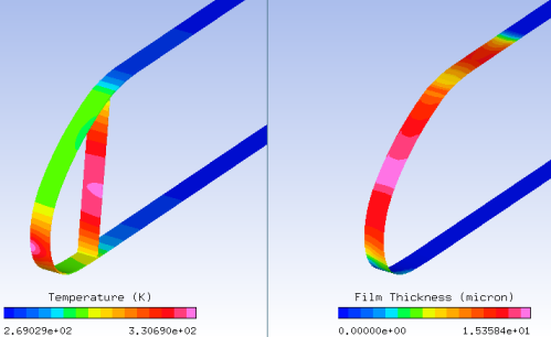
Figure 7.20: Temperature Distribution vs. Wrap Distance on the External Surface for Dry and Wet Air Runs (Z = 0.0001 m)
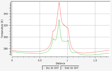
The effect of droplets cooling the surface is clearly visible in the above graph. The wet air surface temperatures are significantly lower than the dry air. Some parts of the wet surface are below the freezing temperature, indicating possible ice formation past the protected zone limits. This will be later verified by running an ICE3D calculation using the results of this CHT simulation.
If ice is expected to form during a CHT simulation (due to insufficient heating or as expected by the design), you should impose a sand-grain roughness over the contaminated surfaces. In this manner, the shape and the thickness of the ice will be more accurately represented over these zones. In CHT3D, this is done by enabling the surface roughness option in the main configuration window. Since roughness changes the turbulence and velocity profiles which consequently change the heat fluxes and shear stresses, the full Navier-Stokes equation should be solved on the external domain during CHT iterations. This option is computationally more expensive than the customary Energy-only CHT3D computation and therefore is necessary only if a more realistic post-CHT ice growth simulation is required. The roughness will be applied only in regions where the instantaneous ice growth rate is non-zero, while the rest of the surface remains smooth.
Create a new CHT3D run and name it
CHT3D_wet_with_Roughness. The CHT configuration window will prompt for the type of CHT simulation desired. Select Piccolo (2 fluids, 1 solid) in the Problem type pull-down menu and then choose the Wet air option. Click the button to continue with the set-up. A set of coupled FENSAP, ICE3D and C3D runs will appear in the run window.Drag & drop the config icon of CHT3D_wet onto the config icon of the main CHT3D_wet_with_Roughness run, and click Full copy button. This will copy all the necessary input files and parameters for the current simulation.
Double-click the main config icon of CHT3D_wet_with_Roughness to activate the roughness option.
Go to the Parameters panel. Set the Number of CHT iterations to
30and Solution output every0iterations (default value).Choose the Solve full Navier-Stokes option in the Flow solver mode – external pull-down menu.
Click the Ice roughness check box to activate the ice roughness option and enter
0.0005meters (default value). For the Flow solver mode – internal, keep the default option Solve energy only.and the current run settings.
Double-click the fluid_ext config icon. Go to Solver panel and change the CFL number from
20000to100and Maximum number of time steps from10to50. Close and save this configuration.Right-click the main config icon of CHT3D_wet_with_Roughness. Select the option in the menu to launch the CHT3D calculation. Use
4or more CPUs for all solvers if possible.From the heat transfer point of view on the protected zone, there is not much difference between this case and the previous one. The actual difference will be visible when the ice shape after CHT is computed in the next two tutorials.
The goal of this simulation is to compute the post-CHT ice shape using the steady-state anti-icing heat fluxes computed in the CHT3D run.
Create a new ICE3D run and name it
ICE3D_post_CHT.Drag & drop the config icon of the ice_ext run of the CHT3D_wet onto the config icon of the current run. This operation automatically links the air and droplet solutions, heat fluxes, grid of the external domain and the reference conditions into the ICE3D_post_CHT run.
Double-click the config icon to edit the input parameters.
Go to the Solver panel. Keep the Automatic time step option enabled and change the Total time of ice accretion to
2400seconds.Run the calculation. Use
4or more CPUs if possible.
In this tutorial, you will look at residual ice accretion when roughness is enabled in the CHT3D run. Roughness is applied only in the regions where instantaneous ice accretion is non-zero.
Create a new ICE3D run and name it
ICE3D_post_CHT_with_Roughness.Drag & drop the config icon of the ice_ext run of the CHT3D_wet_with_Roughness onto the config icon of the current run. (If for any reason the file links appear broken, they can be set manually.)
Double-click the config icon to edit the input parameters.
Go to the Solver panel. Keep the Automatic time step option enabled and change the Total time of ice accretion to
2400seconds.In the Out panel, enable the Generate displaced grid option to get the iced grid for additional flow computations (optional).
Run the calculation. Use
4or more CPUs if possible.To compare the ice shapes obtained with and without roughness, first load the ice shape of Ice Accretion After CHT . Go back to the project window and right-click the swimsol icon of ICE3D_post_CHT run. Choose and load it in a new window. Next, click the View ICE button of the current run and Append. The two grids should be loaded with the ice shapes on them. Split the screen to put the data sets on either sides of the view.
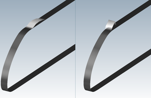
The ice shape with roughness is slightly thicker towards the front of the ice shape as roughness increases cooling effects. This ice shape is an example of ridge ice that can form behind protected zones. In this case it forms due to runback, since ice is located past the impingement limits.
Figure 7.22: Residual Ice Shapes Accreted for 2400 Seconds with the IPS Turned on, without (Left) and with (Right) Roughness
To view the displaced external flow grid, click View in the current run’s execution window, and choose Displaced grid.
The displaced grid can be used for aerodynamic performance analysis to see the adverse effects of the residual ridge ice.
In this tutorial, the residual ice accretion on the nacelle is calculated using the multishot icing methodology, in contrast to the single shot approach employed in Ice Accretion After CHT with Roughness. The multishot icing approach captures the effect the ice shape has on the local airflow and droplet field during the accretion process. This may allow additional phenomena to be captured during the icing process, such as changes in airflow patterns, collection efficiency and shadow zones, etc. However, this approach is more computationally expensive.
Note: In this case, you are using the standard MULTI-FENSAP sequence.
Create a new Sequence → MULTI-FENSAP run and name it
MULTI-FENSAP_post_CHT_with_roughness.Drag & drop the main config icon of the CHT3D_wet_with_Roughness onto the main config icon of the current run. A message will pop up to say that required inputs will be imported from the CHT simulation. Click .
Double-click the fensap config icon to edit the FENSAP solver input parameters. Go to the Solver panel. Set the CFL number to
100and the Maximum number of time steps to300. Close and save the fensap configuration. Uncheck the Use variable relaxation option.Double-click the drop config icon to edit the droplet solver input parameters. Go to the Solver panel. Set the CFL number to
20and the Maximum number of time steps to300. Close and save the drop configuration.Double-click the ice config icon to edit the ICE3D solver input parameters.
In the Model panel, under Icing model, set the Roughness output to CHT constant roughness to maintain the same roughness height computed in your CHT3D with roughness simulation.
Go to the Solver panel. Keep the Automatic time step option enabled and change the Total time of ice accretion to
960seconds.In the Out panel, change the Time between solution output to
960seconds. Close and save the ice configuration.Double click the main config icon to edit the multishot parameters. Click Add iteration twice so that 3 iterations are listed in the table. Change the ice – Total time to
480seconds for Iteration 01, and to960seconds for Iteration 02 and Iteration 03, as shown in the figure below.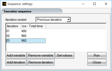
Run the calculation. It’s recommended to use 4 or more CPUs if possible.
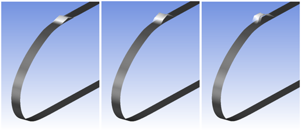
Use Viewmerical to investigate the ice shape as it develops over the 3 shots of ice accretion. Click View Ice of the current run and select -All files-. Go to the Data panel and set the step under Files → Step to
1,2and3to view the ice at the end of each shot of ice accretion. Alternatively, use the slider or click the button move through the shots in sequence.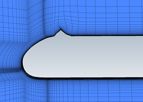
This ice shape is an example of a ridge ice that can form behind protected zones. In this case, it forms due to water runback, since ice is located past the impingement limits. After each shot, additional water runs back along the nacelle towards the ridge of ice and freezes towards the front of the ice shape. The ice obstruction prevents the water from moving further downstream.
Figure 7.23: 3D Views of the Residual Ice Shapes Accreted After 480 (Left), 1440 (Middle) and 2,400 (Right) Seconds with the IPS Turned On, Using a Post CHT Multishot Simulation with Roughness
This tutorial illustrates the procedure to compute the Conjugate Heat Transfer (CHT) through the metal skin of a leading edge, which separates the cold wet air flowing over the external skin surface from the hot internal air flow induced by the jet discharging from the orifice of the piccolo tube. A hot jet from the orifice of a piccolo tube heats the inner skin of the leading edge to prevent ice accretion on the outer surface. In this simulation Fluent, DROP3D and ICE3D will be used to simulate the external flow conditions. C3D simulates the heat conduction through the solid leading edge skin and Fluent will be used to simulate the internal flow.
This tutorial has the same flow conditions as Piccolo Tube Operating in the Wet Air Regime (Anti-Icing) for both external and internal flow domains and consists of the following sequential steps.
Compute the external cold air flow, using Fluent.
Compute the internal hot air flow, using Fluent.
Compute the external droplet impingement (constant source of droplets).
Compute an initial water film on the surface (for a few seconds only).
Conjugate heat transfer across all domains (without Fluent roughness option enabled).
Conjugate heat transfer across all domains (with Fluent roughness option enabled).
Compute ice accretion after CHT (without Fluent roughness option enabled).
Compute ice accretion after CHT (with Fluent roughness option enabled).
Using FENSAP-ICE, create a new project and name it
PICCOLO_FLUENT. Select the metric unit system. Close FENSAP-ICE.Go to the project folder, PICCOLO_FLUENT, and create a new sub folder called INITIAL-AIR. Copy the provided Fluent case file, FLUENT-piccolo-ext.cas.h5, from the tutorials subdirectory ../workshop_input_files/Input_Grid/CHT to this new folder and launch Fluent.
Note: In Windows, Fluent can be launched by going to Start → All Programs → ANSYS 2024 R2 → Fluid Dynamics → Fluent 2024 R2.
In the Fluent Launcher window, select the Dimension as 3D, pick Double Precision under Options, and choose Parallel (Local Machine) under Processing Options. Assign a number of CPUs for this simulation,
2to4CPUs, under Solver → Processes. Click Show More Options. Under General Options, set your Working Directory to the INITIAL-AIR directory. Press to close the Fluent Launcher.Note: Select Serial under Processing Options to run the simulation using a single processor or CPU if multiple processes are not available.
Read the case file by going to the → → menu and browse to and select the Fluent case file, FLUENT-piccolo-ext.cas.h5, located inside the sub folder INITIAL-AIR.
From the top navigation menu, select Physics. Make sure the Solver is set to Pressure-Based, Absolute, and Steady. Click the Operating Conditions. Set the Operating Pressure to
0Pa. Press to close the Operation Conditions window.Expand the Setup → Material → Fluid from the side tree menu. Double-click air and modify its properties. The table below describes the air properties to be imposed in this simulation.
Density Ideal-gas Cp 1004.688J/kg-KThermal Conductivity 0.02325338W/m-KViscosity 1.667512e-05kg/m-sMolecular Weight 28.966kg/kgmolClick the button and this window to save the new air properties.
Expand and double-click Setup → Models → Energy from the side tree menu. Ensure that Energy is turned on.
Expand and double-click Setup → Models → Viscous from the side tree menu. Select the k-omega (2 eqn) option in the opened Viscous Model interface and then select k-omega Model → SST. Make sure that Viscous Heating and Production Limiter are activated in the Options section. In the Model Constants section, drag the scroll bar down and set Energy Prandtl Number and Wall Prandtl Number values to
0.9. Click to close this menu.Expand and double-click Setup → Boundary Conditions from the side tree menu. Set the interior-2 boundary to interior.
In the Task Page → Boundary Conditions list, click the pressure-far-field-4 and then select pressure-far-field from the drop-down list of Type. Click Edit to open the Pressure Far-Field window and set the following conditions for this boundary:
Momentum panel
Gauge Pressure 101325PaMach Number 0.15692X, Y, and Z-Components of Flow Direction 1,0and0Turbulence Specification Method Intensity and Viscosity Ratio Turbulence Intensity 0.08%Turbulent Viscosity Ratio 1e-05Thermal panel
Temperature 263.15K (-10 °C)Repeat this step for the pressure-far-field-5 boundary.
In the Task Page → Boundary Conditions list, click the pressure-outlet-8 and select pressure outlet from the drop-down list of Type. Set the following for this boundary:
Momentum panel
Gauge Pressure 101325PaTurbulence Specification Method Intensity and Viscosity Ratio Backflow Turbulence Intensity 0.08%Backflow Turbulent Viscosity Ratio 1e-05Thermal panel
Backflow Total Temperature 264.446K
In the Task Page → Boundary Conditions list, click the symmetry-9 boundary and select symmetry from the drop-down list of Type
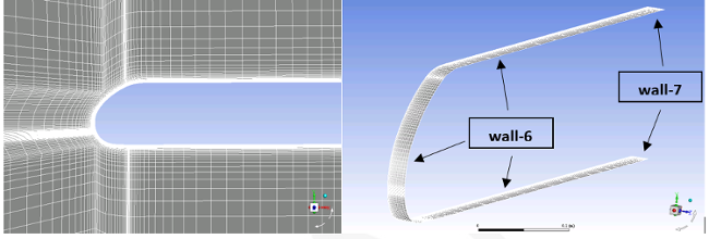
In the Task Page → Boundary Conditions list, double-click the wall-6 to open Wall window. In the Momentum panel, set the Wall Motion to Stationary Wall and the Shear Condition to No Slip. In the Thermal panel, set the Thermal Conditions to a Temperature of
274.446K. Click to close the window. Repeat this step for wall-7 boundary.Expand and double-click Setup → Reference Values from the side tree menu. In the Task Page, use the Compute from drop-down menu to select pressure-far-field-5.
Expand and double-click Solution → Methods from the side tree menu. Set the Pressure-Velocity Coupling section to Coupled. In the Spatial Discretization section, set the Gradient to Green-Gauss Cell Based and the remaining settings to Second Order or Second Order Upwind. Enable High Order Term Relaxation with its Options to All Variables and Relaxation Factor to
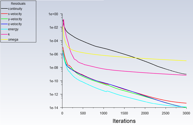
0.25.Expand and double-click Solution → Monitors → Residual from the side tree menu. In the Residual Monitors window, make sure that the Print to Console and the Plot are enabled. Disable all check box below the Convergence column. Close this window once this is done.
Expand and double-click Solution → Report Definitions from the side tree menu. In the opened Report Definitions window, do the following:
Click and select New → Force Report → Lift to open the Lift Report Definition window. Change the Name to
report-def-cl. Click to select wall-6 and wall-7 on the list box below Wall Zones. Enable Report File and Print to Console under Create and set Frequency value to1. Click to close the Lift Report Definition window.Click and select New → Force Report → Drag to open the Drag Report Definition window. Change the Name to
report-def-cd. Click to select wall-6 and wall-7 on the list box below Wall Zones. Enable Report File and Print to Console under Create and set Frequency value to1. Click to close the Drag Report Definition window.Click and select New → Surface Report → Integral to open Surface Report Definition window. Change the Name to
report-def-heat. Set the Field Variable to Wall Fluxes → Total Surface Heat Flux. Click to select wall-6 and wall-7 on the list box below Surfaces. Enable Report File and Print to Console under Create and set Frequency value to1. Click to close the Surface Report Definition window.
Click to close the Report Definitions window.
Expand and double-click Solution → Initialization from the side tree menu. In the opened Task Page, select Hybrid Initialization under Initialization Methods. Click the button to initialize the computational domain.
Expand and double-click Solution → Run Calculation from the side tree menu. Enter
3000as the total Number of Iterations and click Calculate to start the simulation.Once the simulation is complete, save the new Fluent solutions in → → . Name this simulation as
FLUENT-piccolo-ext.cas.h5/dat.h5.The following figure shows the convergence history of the external airflow simulation with Fluent:
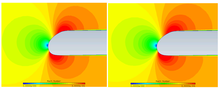
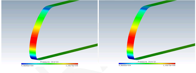
The following figures compare the Fluent solution to a FENSAP kw-sst airflow solution.
Note: To appropriately compare the results of this CHT anti-icing simulation using Fluent with the kw-sst turbulence model, another CHT anti-icing simulation using FENSAP-ICE with its own kw-sst turbulence model was conducted. Piccolo Tube Operating in the Wet Air Regime (Anti-Icing) uses the Spalart-Allmaras turbulence model and therefore its results are not suitable to make proper comparisons. Results and comparisons of both kw-sst cases are presented throughout this tutorial and show that Fluent and FENSAP-ICE produce similar CHT results.
Copy the Fluent case file, FLUENT-piccolo-int.cas.h5, from the tutorials subdirectory ../workshop_input_files/Input_Grid/CHT to the INITIAL-AIR folder.
Select → → from the Fluent main menu. Navigate to INITIAL-AIR and select the file, FLUENT-piccolo-int.cas.h5, to open the internal case file with Fluent.
From the top navigation menu, select Physics. Make sure the Solver is set to Pressure-Based, Absolute, and Steady. Click the Operating Conditions.... Set the Operating Pressure (pascal) to
0Pa. Press to close the Operation Conditions window.Expand Setup → Material → Fluid from the side tree menu. Double-click air and modify its properties. The table below describes the air properties to be imposed in this simulation.
Density Ideal-gas Cp 1004.688J/kg-KThermal Conductivity 0.02830653W/m-KViscosity 2.010212e-05kg/m-sMolecular Height 28.966kg/kgmolClick the button and this window to save the new air properties.
Expand and double-click Setup→ Models → Energy from the side tree menu. Make sure that Energy is turned on.
Expand and double-click Setup → Models → Viscous from the side tree menu. Select the k-omega (2 eqn) option in the opened Viscous Model interface and then select k-omega Model → SST. Make sure that Viscous Heating and Production Limiter are activated in the Options section. In the Model Constants section, drag the scroll bar down and set Energy Prandtl Number and Wall Prandtl Number values to
0.9. Click to close this menu.Expand and double-click Setup → Boundary Conditions from the side tree menu. Set the interior-2 boundary to interior.
In the Task Page → Boundary Conditions list, click the velocity-inlet-4 and then select velocity-inlet from the drop-down list of Type. Click Edit to open the velocity-inlet window and set the following conditions for this boundary:
Momentum panel
Velocity Specification Method Magnitude and Direction Reference Frame Absolute Velocity Magnitude 367.2557m/sSupersonic/Initial Gauge Pressure 101502.4PaCoordinate System Cartesian (X, Y, Z) X, Y, Z-Components of Flow Direction -0.9396926, -0.3420201and0Turbulence Specification Method Intensity and Viscosity Ratio Turbulence Intensity 0.08%Turbulent Viscosity Ratio 1e-05Thermal panel
Temperature 335.4K (62.25°C)These conditions specify an orifice velocity with a Mach number slightly above 1. The velocity vector is perpendicular to the inlet.
In the Task Page → Boundary Conditions list, click the pressure-outlet-8 and select pressure-outlet from the drop-down list of Type. Set the following for this boundary:
Momentum panel
Gauge Pressure 101325PaTurbulence Specification Method Intensity and Viscosity Ratio Backflow Turbulence Intensity 0.08%Backflow Turbulent Viscosity Ratio 1e-05Thermal panel
Backflow Total Temperature 335K (61.85°C)
In the Task Page → Boundary Conditions list, click the symmetry-9 boundary and select symmetry from the drop-down list of Type.
In the Task Page → Boundary Conditions list, double-click the wall-5 to open Wall window. In the Momentum panel, set the Wall Motion to Stationary Wall and the Shear Condition to No Slip. In the Thermal panel, set the Thermal Conditions to Temperature at
320K (46.85°C). Click to close the window. Repeat this step for wall-7 boundary.In the Task Page → Boundary Conditions list, double-click the wall-6 to open the Wall window. In the Momentum panel, set the Wall Motion to Stationary Wall and the Shear Condition to No Slip. In Thermal panel, set the Thermal Conditions to Heat Flux to
0W/m2. Click to close the window.Note: Temperature must be specified on the interfacing boundary condition families to initiate the heat transfer between the two domains (air and solid). In this case wall-5 will be interfacing with the leading edge part of the solid, and wall-7 will interface with the back plate. These temperatures will be updated automatically during the CHT3D loop, as conduction takes place in the solid.
Expand and double-click Setup → Reference Values from the side tree menu. In the Task Page, use the Compute from drop-down menu to select velocity-inlet-4. Set the Length to
0.05m.Expand and double-click Solution → Methods from the side tree menu. Set the Pressure-Velocity Coupling section to Coupled. In the Spatial Discretization section, set the Gradient to Green Gauss Node Based and the remaining settings to Second Order or Second Order Upwind. Enable Pseudo Transient and High Order Term Relaxation, with its Options to All Variables and Relaxation Factor to
0.25.Expand and double-click Solution → Monitors → Residual from the side tree menu. In the Residual Monitors window, make sure that the Print to Console and the Plot are enabled. Disable all check box below the Convergence column. Close this window once this is done.
Expand and double-click Solution → Report Definitions from the side tree menu. In the opened Report Definitions window, click and select New → Surface Report → Integral to open Surface Report Definition window. Change the Name to
surf-heatflux-rset. Set the Field Variable to Wall Fluxes → Total Surface Heat Flux. Click to select wall-5 on the list box below Surfaces. Enable Report File and Print to Console under Create and set Frequency value to1. Click to close the Surface Report Definition window. Then, click in the Report Definitions window to save the configurations.Expand and double-click Solution → Initialization from the side tree menu. In the opened Task Page, select Hybrid Initialization under Initialization Methods. Click the button to initialize the computational domain.
Expand and double-click Solution → Run Calculation from the side tree menu. Enter
5000as the total Number of Iterations and click Calculate to start the simulation.Once the simulation is complete, save the new Fluent solutions in → → . Name this simulation as FLUENT-piccolo-int.cas.h5/dat.h5.
Click → from the main menu to close Fluent.
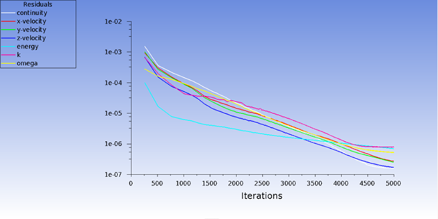
The following figure shows the convergence history of the internal airflow simulation with Fluent:


Open the PICCOLO_FLUENT project with FENSAP-ICE. Use the → menu or the new run icon to create a new DROP3D run. Name this run
DROP3D_ext_FLUENT.Right-click the grid icon and select Define. Navigate to the folder, INITIAL-AIR, and select, FLUENT-piccolo-ext.cas.h5. Then press Open and a new Grid converter window appears. Accept the default options and click or Next.
The Grid converter will now execute. When done, click Finish. Fluent icons will now appear in the grid and airsol input sections to the left of the config icon.
Double-click the DROP3D_ext_FLUENT config icon to edit the input parameters.
Go to the Conditions panel and check that the following Droplet reference conditions have been set by default:
Liquid Water Content 1g/m3Droplet diameter 20micronsWater density 1000kg/m3Go to Boundaries panel. Select the BC_1000 and BC_1001 (Inlet) boundary condition and click Import reference conditions.
Go to the Solver panel. Set the CFL number to
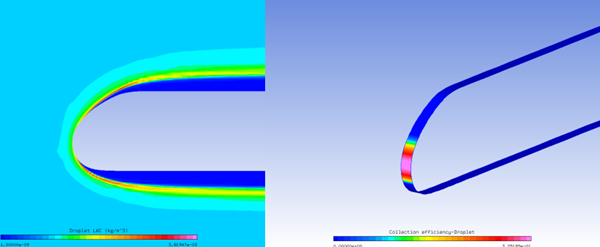
20and the Maximum number of time steps to300. Click the button. Start the calculation on4or more CPUs if possible.The following figures show the computed liquid water content and collection efficiency and compare these results against a DROP3D solution computed from a FENSAP kw-sst airflow.
Note: To appropriately compare the results of this CHT anti-icing simulation using Fluent with the kw-sst turbulence model, another CHT anti-icing simulation using FENSAP-ICE with its own kw-sst turbulence model was conducted. Piccolo Tube Operating in the Wet Air Regime (Anti-Icing) uses the Spalart-Allmaras turbulence model and therefore its results are not suitable to make proper comparisons. Therefore, results and comparisons of both kw-sst cases are presented throughout this tutorial and show that Fluent and FENSAP-ICE produce similar CHT results.

The goal of this step is not to provide an initial ice shape, but rather to establish a water film on the outer surface of the solid as an initial condition for the wet CHT run.
Create a new ICE3D run and name it
ICE3D_ext_FLUENT.Drag & drop the config icon of DROP3D_ext_FLUENT onto the config icon of this new run. This operation automatically links the air and droplet solutions, the grid of the external domain and the reference conditions into the ICE3D_ext_FLUENT run.
Double-click the config icon to edit the input parameters.
Go to the Model panel. Change the Icing model to Glaze - Advanced and select Classical in Heat flux type.
Go to the Conditions panel. Set the Recovery factor to
0.9.Go to the Solver panel. Keep the Automatic time step option enabled and change the Total time of ice accretion to
30seconds.Run the calculation on
4or more CPUs if possible.
Create a new CHT3D run and name it
CHT3D_wet_FLUENT. The CHT configuration window will appear to prompt for the type of CHT simulation desired. Select Piccolo (2 fluids, 1 solid) in the Problem type pull-down menu, then choose Wet air. Select FLUENT in the Flow Solver (External) and (Internal) settings. Press the button to continue with the setup. A tree of coupled Fluent, ICE3D and C3D runs will appear in the run window.Right-click the grid icon of fluid_ext and select Define. Navigate to the INITIAL-AIR folder and select the FLUENT-piccolo-ext.cas.h5 file. Then press Open and a new Grid converter window appears. Accept the default options and click or Next. Once the grid and solution conversions are completed, click the Finish button to close this window.
Double-click the config icon of the fluid_ext run to edit the input parameters. In the FLUENT configuration window, do the following:
Set the Number of iterations to
50;Set the correct path to the FLUENT executable;
Set the launch Parameters to “3ddp -t$NCPU -g -i $JOURNAL -wait”.
Click to close the FLUENT configuration window.
Drag & drop the config icon from ICE3D_ext_FLUENT onto the config icon of the ice_ext run in CHT3D_wet_FLUENT.
Right -click the grid icon of fluid_int and select Define. Navigate to the INITIAL-AIR folder and select the FLUENT-piccolo-int.cas.h5 file. Press Open and a new Grid converter window appears. Accept the default options and click or Next. Once the grid and solution conversions are completed, click Finish to close this window.
Note: When the Reference parameters table appears in the Grid converter window, double-check and make sure that the magnitude of the velocity vector (compute this value using the X, Y, and Z-velocity component) is equal to the Value of the Reference velocity.
Double-click the config icon of the fluid_int run to edit the input parameters. In the FLUENT configuration window, do the following:
Set the Number of iterations to
50;Set the correct path to the FLUENT executable;
Set the launch Parameters to “3ddp -t$NCPU -g -i $JOURNAL -wait”.
Click to close the FLUENT configuration window.
To set up the solid run in CHT3D_wet_FLUENT, double-click the grid_material icon and select the file grid_solid provided under the tutorials subdirectory CHT.
Go to the Settings panel. Set the Temperature value to
300K (26.85°C). This will be the initial temperature throughout the solid domain.Go to the Properties panel. Click the Rename button to change the material name from default to
duralumin. Specify the following characteristics for the material:Density 2787kg/m3Conductivity 164W/m/KEnthalpy 241060J/kgGo to the Materials panel. Since duralumin is the only material in the solid domain, the label MAT_0 will be automatically assigned to it.
Go to the Boundaries panel. Define the boundary conditions of the outer surfaces of the solid as follows:
BC_2001: Default settings (Thermal BC definition set to Nothing)
BC_2002: Default settings (Thermal BC definition set to Nothing)
BC_2004: Default settings (Thermal BC definition set to Nothing)
BC_2005: Select a Neumann condition, set Heat flux to
0W/m2BC_2006: Set Thermal BC definition to Type: Flux, and set Heat flux to
0W/m2/KBC_2007: Set Thermal BC definition to Type: Flux, and set Heat flux to
0W/m2/KBC_4100: Set Thermal BC definition to Type: Flux, and set Heat flux to
0W/m2/KBC_4300: Set Thermal BC definition to Type: Flux, and set Heat flux to
0W/m2/K
Note: CHT3D will automatically update the boundary conditions on BC_2001, BC_2002, and BC_2004 during the simulation.
Go to the Solver panel. Select Constant from the drop-down menu of Time step. Set the Time step value to
0.1seconds and the Total time to5seconds. At each CHT3D iteration, heat conduction will be computed for 5 seconds. Close and save this configuration.Double-click the main config icon of CHT3D_wet_FLUENT to set up the links between the solid and fluid domains.
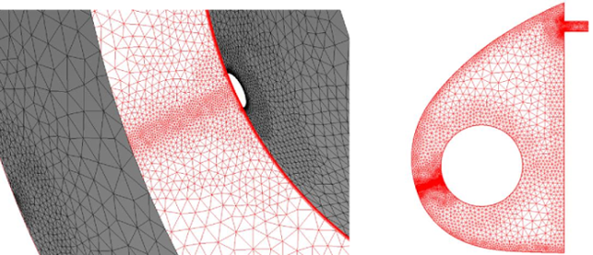
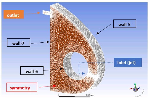
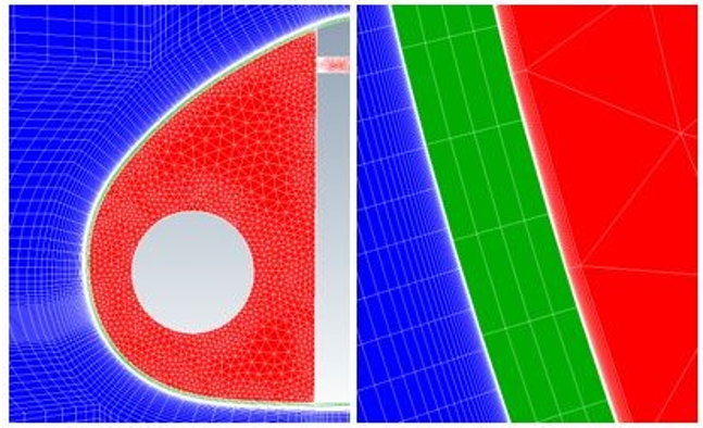
Figure 7.38: The 3 Computational Domains: Blue (External), Red (Internal), Green (Solid). Right: Stagnation Point
Go to the Parameters panel. Set the Number of CHT iterations (loops) to
30and Solution output every0seconds (default value).Choose the Solve full Navier-Stokes option in the Flow solver mode pull-down menu for both external and internal flow.
Note: Unlike CHT3D with FENSAP, CHT3D with Fluent does not support the Solve energy only option.
Go to the Interfaces panel. There are three fluid/solid interfaces in the computational domain. CHT3D will automatically exchange the boundary conditions between these three interfaces. Set up the interfaces as follows:
For External to Solid: There is only one interface between the external domain and the solid. Set the interface boundaries as follows:
External fluid grid: 2001: wall-6
Solid grid: 2001
For Solid to Internal: There are two interfaces between the solid and the internal domain. Set the first interface as follows:
Solid grid: 2002
Internal fluid grid: 2000: wall-5
Then click
next to Interface label to add the third interface and set it as
follows:Solid grid: 2004
Internal fluid grid: 2002: wall-7
Go to the Temperatures panel. Set the External Surface recovery temperature to
264.316K (-8.834°C). Set the Internal adiabatic stagnation temperature to402.52K (129.37°C).Note: The value of the External Surface recovery temperature is computed by applying a recovery factor of 0.9 on the total temperature of the external airflow. The value of the Internal adiabatic stagnation temperature is the total air temperature at the jet hole of the internal domain. Both values are used as reference temperatures, for the external and internal domains respectively, during a CHT simulation.
Close and save the configuration.
Right-click the main config icon of CHT3D_wet_FLUENT, then select the option in the menu to launch the CHT3D calculation. Use
4or more CPUs for all solvers if possible, and launch the calculation.This simulation takes a substantial amount of time to complete.
Figure 7.39: Convergence History of the Maximum Solid Wall Temperatures (Left: Fluent; Right: FENSAP kw-sst - Energy Only)
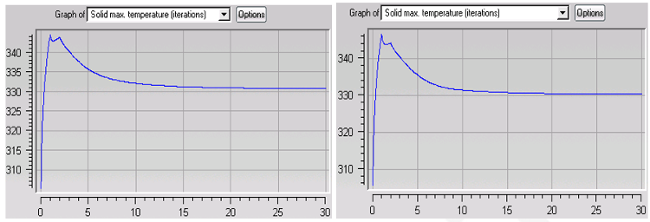
Figure 7.40: Convergence History of the Minimum (Right) Solid Wall Temperatures (Left: Fluent; Right: FENSAP kw-sst – Energy Only)
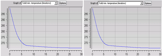
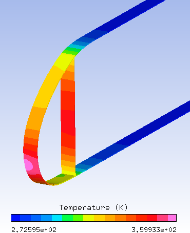
Figure 7.41: Temperature Contours on the Solid (C3D) (Left: Fluent; Right: FENSAP kw-sst – Energy Only)
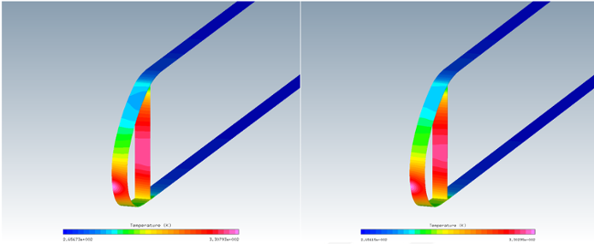
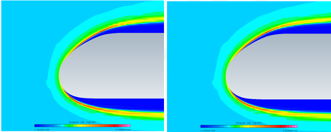
Figure 7.42: Water Film Thickness on the External Surface (ICE3D) (Left: Fluent; Right: FENSAP kw-sst – Energy Only)
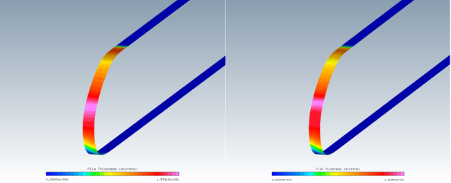
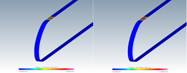
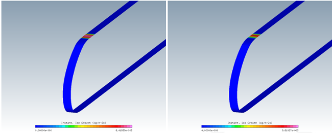
Figure 7.43: Instantaneous Ice Growth on the External Surface (ICE3D) (Left: Fluent; Right: FENSAP kw-sst – Energy Only)
If ice is expected to form during a CHT simulation (due to insufficient heating or as designed), you should impose a sand-grain roughness over the contaminated surfaces. In this manner, the shape and the thickness of the ice will be more accurately represented over these zones. In CHT3D, this is done by enabling the surface roughness option in the main configuration window. Since roughness changes the turbulence and velocity profiles which consequently change the heat fluxes and shear stresses, the full Navier-Stokes equation should be solved on the external domain during CHT iterations. Roughness will be applied only in regions where the instantaneous ice growth rate is non-zero, while the rest of the surface remains smooth.
Create a new CHT3D run and name it
CHT3D_wet_FLUENT_with_roughness. The CHT configuration window will appear to prompt for the type of CHT simulation desired. Select Piccolo (2 fluids, 1 solid) in the Problem type pull-down menu, then choose Wet air. Select FLUENT in the Flow Solver (External) and (Internal) settings. Click to continue with the setup. A tree of coupled Fluent, ICE3D and C3D runs will appear in the run window.Drag & drop the config icon of CHT3D_wet_FLUENT onto the config icon of the main CHT3D_wet_FLUENT_with_roughness run, and click Full copy button. This will copy all the necessary input files and parameters for the current simulation.
Double-click the main config icon of CHT3D_wet_FLUENT_with_Roughness to activate the roughness option.
Go to the Parameters panel. Set the Number of CHT iterations to
30and Solution output every0iterations (default value).Choose the Solve full Navier-Stokes option in the Flow solver mode – external pull-down menu.
Click the Ice roughness check box to activate the ice roughness option and enter
0.0005meters (default value). Choose the Solve full Navier-Stokes option in the Flow solver mode – internal pull-down menu.Click and Save the current run settings.
Right-click the main config icon of CHT3D_wet_FLUENT_with_Roughness. Select the option in the menu to launch the CHT3D calculation. Use
4or more CPUs for all solvers if possible.Figure 7.44: Temperature Contours on the Solid (C3D) (Left: Fluent; Right: FENSAP kw-sst – Full Navier-Stokes)
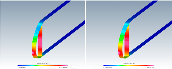
Figure 7.45: Water Film Thickness on the External Surface (ICE3D) (Left: Fluent; Right: FENSAP kw-sst – Full Navier-Stokes)
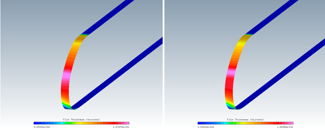
Figure 7.46: Instantaneous Ice Growth on the External Surface (ICE3D) (Left: Fluent; Right: FENSAP kw-sst – Full Navier-Stokes)
From the heat transfer point of view on the protected zone, there is not much difference between this case and the previous one. The actual difference will be visible when the ice shape after CHT is computed in the next sections.
After the CHT computation is complete, the rate at which ice will accrete can be assessed by looking at the Instantaneous Ice Growth data field in the ICE3D solution file swimsol. However, the amount of ice can be visualized by performing a post-CHT ICE3D simulation.
Create a new ICE3D run and name it
ICE3D_post_CHT_FLUENT.Drag & drop the config icon of the ice_ext section of the CHT3D_wet_FLUENT simulation onto this new ICE3D run. This operation automatically links the air and droplet solutions, heat fluxes, grid of the eternal domain and the reference conditions into the ICE3D_post_CHT_FLUENT.
Double-click the config icon to edit the input parameters.
Go to the Solver panel. Keep the Automatic time step option enabled and change the Total time of ice accretion to
2400seconds.Go to the Out panel. Set the Time between solution output to
2400seconds. This will only output and write the final solution.Run the calculation. Use
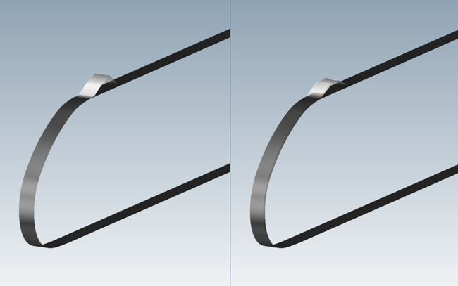
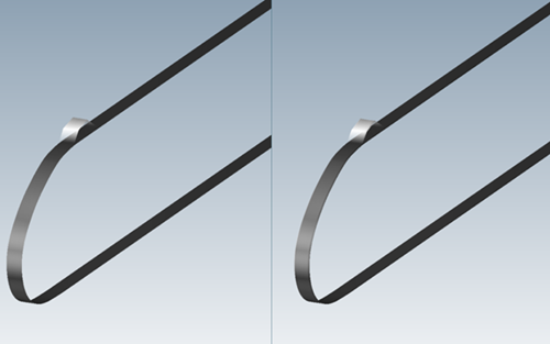
4or more CPUs if possibleFigure 7.47: Residual Ice Shape Accreted for 2400 Seconds with the Hot Air IPS Turned On (Left: Fluent; Right: FENSAP kw-sst – Energy Only)
After the CHT computation is done, the rate at which ice will accrete can be assessed by looking at the Instantaneous Ice Growth data field in the ICE3D solution file swimsol. However, the amount of ice can be visualized by performing a post-CHT ICE3D simulation.
Create a new ICE3D run and name it
ICE3D_post_CHT_FLUENT_with_roughness.Drag & drop the config icon of the ice_ext section of the CHT3D_wet_FLUENT_with_roughness simulation onto this new ICE3D run. This operation automatically links the air and droplet solutions, heat fluxes, grid of the external domain and the reference conditions into the ICE3D_post_CHT_FLUENT_with_roughness.
Double-click the config icon to edit the input parameters.
Go to the Solver panel. Keep the Automatic time step option enabled and change the Total time of ice accretion to
2400seconds.In the Out panel, set the Time between solution output to
2400seconds. This will only output and write the final solution. Select Yes from the drop-down menu of the Generate displaced grid option to get the displaced-iced grid for additional flow computations (optional).Run the calculation. Use
4or more CPUs if possible.Note: To compare the ice shapes obtained without and with roughness in CHT, first load the ice shape of ICE3D_post_CHT_FLUENT. Go back to the project window and right-click the swimsol icon of the ICE3D_post_CHT_FLUENT run. Choose and load it in a new window. Next, click the button of the current run and Append. The two grids should be loaded with the ice shapes on them. Split the screen to put the data sets on either sides of the view.
Figure 7.48: Residual Ice Shape Accreted for 2400 Seconds with the Hot Air IPS Turned On (Left: Fluent; Right: FENSAP kw-sst Energy only)
To view the displaced external flow grid, right-click the grid_disp icon of the ICE3D_post_CHT_FLUENT_with_roughness run and select View with VIEWMERICAL.
Note: The displaced grid can be used for performance analysis to see the adverse effects of the residual ridge ice.
Figure 7.49: Displaced External Flow Grid with Residual Ice Obtained by Running ICE3D After CHT (Left: Fluent with Roughness; Right: FENSAP kw-sst with Roughness)
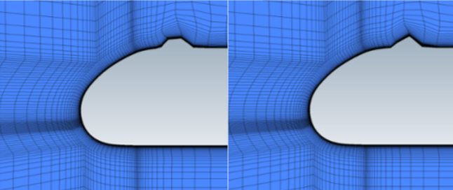
This tutorial illustrates the procedure to compute the Conjugate Heat Transfer (CHT) through the metal skin of a leading edge, which separates the cold wet air flowing over the external skin surface from the hot internal air flow induced by the jet discharging from the orifice of the piccolo tube. A hot jet from the orifice of a piccolo tube heats the inner skin of the leading edge to prevent ice accretion on the outer surface. In this simulation CFX, DROP3D and ICE3D will be used to simulate the external flow conditions. C3D simulates the heat conduction through the solid leading edge skin and CFX will be used to simulate the internal flow.
This tutorial has the same flow conditions as Piccolo Tube Operating in the Wet Air Regime (Anti-Icing) for both external and internal flow domains and consists of the following sequential steps.
Compute the external cold air flow, using CFX.
Compute the internal hot air flow, using CFX.
Compute the external droplet impingement (constant source of droplets).
Compute an initial water film on the surface (for a few seconds only).
Conjugate heat transfer across all domains (without CFX roughness option enabled).
Conjugate heat transfer across all domains (with CFX roughness option enabled).
Compute ice accretion after CHT (without CFX roughness option enabled).
Compute ice accretion after CHT (with CFX roughness option enabled).
Using FENSAP-ICE, create a new project and name it
PICCOLO_CFX. Select the metric unit system. Close FENSAP-ICE.Go to the project folder, PICCOLO_CFX, and create a new sub folder called
INITIAL-AIR. Copy the provided CFX file, CFX-piccolo-ext.cfx , from the tutorials subdirectory ../workshop_input_files/Input_Grid/CHT to this new folder and launch CFX-Pre.Note: On Windows, CFX-Pre can be launched by going to → → → .
In the Ansys CFX 2024 R2 Launcher, set the Working Directory to
../PICCOLO_CFX/INITIAL-AIR. Click the CFX-Pre icon below the launcher’s main menu to launch CFX.Click → from Ansys CFX-MeshCFX-Pre’s main menu and select the file CFX-piccolo-ext.cfx to open it in CFX-Pre.
Expand Simulation → Materials under the Outline tree view. Double-click the Air Ideal Gas icon to open the Material: Air Ideal Gas main tab. Go to its sub tab Material Properties and modify the air properties as shown in the table below:
Molar Mass 28.966kg/kgmolSpecific Heat Capacity 1004.688J/kg-KDynamic Viscosity 1.667512e-05kg/m-sThermal Conductivity 0.02325338W/m-KClick then to close the Material: Air Ideal Gas tab and save the new air properties.
Note: Thermal conductivity and viscosity are computed from these equations which are presented in the FENSAP-ICE User Manual and shown below.


In these equations,
 refers to the ambient air static temperature, and
  ,
,  and
and  are respectively equal to 0.00216176 W/m/K3/2,
288 K and 17.9*10-6 Pa s.
are respectively equal to 0.00216176 W/m/K3/2,
288 K and 17.9*10-6 Pa s.Expand Simulation → Flow Analysis 1 under the Outline tree view. Double-click its sub section Default Domain to open the Domain: Default Domain tab and to edit the domain settings.
In its sub tab Basic Settings, change the Material to and the Reference Pressure to
0Pa.In its sub tab Fluid Models, under Heat Transfer, set the Option to and enable Incl. Viscous Work Term. Under Turbulence, set the Option to .
Click then to save the new settings and close the main tab.
Expand Simulation → Flow Analysis 1 → Default Domain to set boundary conditions of the domain:
Double-click to edit the farfield boundary condition.
Under the Basic Settings tab, set the Boundary Type to . Hold the Ctrl key to select the and from the drop-down box of Location.
Under the Boundary Details tab,
Set the Flow Regime Option to .
Set the Mass and Momentum Option to with [U, V, W] components of [
51.03,0,0] m/s.Set Turbulence Option to with a Fractional Intensity of
0.0008and an Eddy Viscosity Ratio of1e-5.Set the Heat Transfer Option to and the to
263.15K.
Click then to save the settings and close the main tab.
Double-click to edit the outlet boundary condition.
Under the Basic Settings tab, set the Boundary Type to . Select the from the drop-down box of Location.
Under the Boundary Details tab, set the Flow Regime Option to . Set the Mass and Momentum Option to and the Relative Pressure to
101 325Pa.
Click then to save the settings and close the main tab.
Double-click to edit the wall_cht boundary condition.
Under the Basic Settings tab, set the Boundary Type to . Select from the drop-down box of Location.
Under the Boundary Details tab, set the Mass and Momentum Option to , Wall Roughness Option to , and Heat Transfer Option to with a Fixed Temperature value of
274.446K.
Click then to save the settings and close the main tab.
Double-click to edit the wall_end boundary condition.
Under the Basic Settings tab, set the Boundary Type to . Select from the drop-down box of Location.
Under the Boundary Details tab, set the Mass and Momentum Option to , Wall Roughness Option to , and Heat Transfer Option to with a Fixed Temperature value of
274.446K.
Click then to save the settings and close the main tab.
Double-click to edit the symmetry boundary condition. In the Basic Settings tab, set the Boundary Type to . Select from the drop-down box of Location.
Click then to save the settings and close the main tab.
Expand Simulation → Flow Analysis 1 → Solver and double-click to edit the Solver Control. Under its sub tab Basic Settings, do the following:
Set the Advection Scheme Option and Turbulence Numerics Option to ;
Under Convergence Control, set the Min. Iterations to
1and Max. Iterations to1000;Under Fluid Timescale Control, set the Timescale Control to , Length Scale Option to , and Timescale Factor to a value of
1;Under Convergence Criteria, set the Residual Type to and Residual Target to a value of
1e-20.
Click then to save the settings and close the main tab.
Expand Simulation Control and double-click to edit Execution Control. Under its sub tab Run Definition, do the following:
Under the Input File Settings, set the Solver Input File to
CFX-piccolo-ext.def;Under Run Settings, set Type of Run to and enable ;
Under Parallel Environment, set the Run Mode to and assign
4to the Number of Processes.
Click then to save the settings and close the main tab.
Click → from the main menu to save and browse to overwrite the CFX-piccolo-ext.cfx file under the sub folder INITIAL-AIR.
Click the Define Run icon
 from the main tool bar to proceed with the
simulation. Click to bring up the Define Run ,
then to launch the run.
from the main tool bar to proceed with the
simulation. Click to bring up the Define Run ,
then to launch the run.Once the simulation is completed, a new file, CFX-piccolo-ext_001.res, will be automatically saved inside the working directory, ../PICCOLO_CFX/INITIAL-AIR. The following shows the converging history of the external airflow simulation with CFX.
The following figures compare the CFX external airflow solution to FENSAP/Fluent kw-sst airflow solution.
Figure 7.52: Initial External Airflow Results: Mach Number (Left: CFX; Middle: Fluent Launcher.; Right: FENSAP)
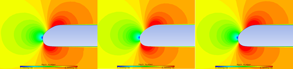
Figure 7.53: Initial External Airflow Results: Surface Pressure (Left: CFX; Middle: Fluent; Right: FENSAP)
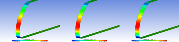
Figure 7.54: Initial External Airflow Results: Surface Shear Stress (Left: CFX; Middle: Fluent; Right: FENSAP)
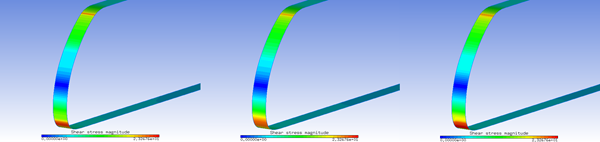
Figure 7.55: Initial External Airflow Results: Surface Heat-flux (Left: CFX; Middle: Fluent; Right: FENSAP)
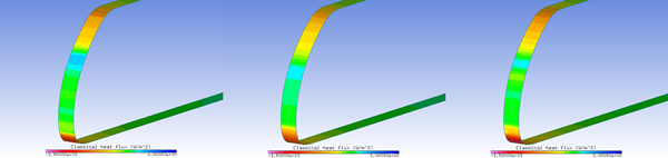
Note: To appropriately compare the results of this CHT anti-icing simulation using CFX with the kw-sst turbulence model, another CHT anti-icing simulation using FENSAP with its own kw-sst turbulence model was conducted. Piccolo Tube Operating in the Wet Air Regime (Anti-Icing) uses the Spalart-Allmaras turbulence model and therefore its results are not suitable to make proper comparisons. Results and comparisons of all kw-sst cases are presented throughout this tutorial and show that CFX and FENSAP/Fluent produce similar CHT results.
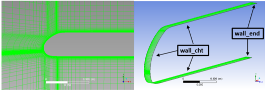
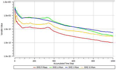
Copy the CFX file, CFX-piccolo-int.cfx, from the tutorial’s subdirectory ../workshop_input_files/Input_Grid/CHT to the INITIAL-AIR folder.
Go back to the Ansys CFX 2024 R2 Launcher. Click the CFX-Pre icon below the main menu to launch CFX-Pre.
Click → from CFX-Pre’s main menu and select the file CFX-piccolo-int.cfx to open it in CFX-Pre.
Expand Simulation → Materials under the Outline tree view. Double-click the Air Ideal Gas icon to open the Material: Air Ideal Gas main tab. Go to its sub tab Material Properties and modify the air properties as shown in the table below:
Molecular Height 28.966kg/kgmolSpecific Heat Capacity 1004.688J/kg-KDynamic Viscosity 2.010212e-05kg/m-sThermal Conductivity 0.02830653W/m-KClick then to close the Material: Air Ideal Gas tab and save the new air properties.
Note: Thermal conductivity and viscosity are computed from these equations which are presented in the FENSAP-ICE User Manual and shown below.
In these equations,
refers to the ambient air static temperature, and , and are respectively equal to 0.00216176 W/m/K3/2,
288 K and 17.9*10-6 Pa s.Expand Simulation → Flow Analysis 1 under the Outline tree view. Double-click its sub section Default Domain to open the Domain: Default Domain tab and to edit the domain settings:
In its sub tab Basic Settings, change the Material to and the to
0Pa.In its sub tab Fluid Models, under Heat Transfer, set the Option to and enable under Turbulence and set the Option to .
Click then to save the new settings and close the main tab.
Expand Simulation → Flow Analysis 1 → Default Domain to set boundary conditions of the domain:
Double-click to edit the inlet boundary condition.
Under the Basic Settings tab, set the Boundary Type to . Select from the drop-down box of Location.
Under the Boundary Details tab:
Set the Flow Regime Option to .
Set the Mass and Momentum Option to Cart. Vel. & Pressure with a Rel. Static Pres. value of
101 502.4Pa and [U, V, W] components of [-345.107471232,-125.608847151,0] m/s.Set Turbulence Option to with a Fractional Intensity of
0.0008and an Eddy Viscosity Ratio of1e-5.Set the Heat Transfer Option to and the Static Temperature to
335.4K.
Click then to save the settings and close the main tab.
Double-click to edit the outlet boundary condition.
Under the Basic Settings tab, set the Boundary Type to . Select the from the drop-down box of Location.
Under the Boundary Details tab, set the Flow Regime Option to . Set the Mass and Momentum Option to and the Relative Pressure to
101 325Pa.
Click then to save the settings and close the main tab.
Double-click to edit the symmetry boundary condition. In the Basic Settings tab, set the Boundary Type to . Select from the drop-down box of Location. Click then to save the settings and close the main tab.
Double-click to edit the wall_adiabatic boundary condition.
Under the Basic Settings tab, set the Boundary Type to . Select from the drop-down box of Location.
Under the Boundary Details tab, set the Mass and Momentum Option to , Wall Roughness Option to , and Heat Transfer Option to .
Click then to save the settings and close the main tab.
Double-click to edit the wall_ext_cht boundary condition.
Under the Basic Settings tab, set the Boundary Type to . Select from the drop-down box of Location.
Under the Boundary Details tab, set the Mass and Momentum Option to , Wall Roughness Option to , and Heat Transfer Option to with a Fixed Temperature value of
320K.
Click then to save the settings and close the main tab.
Double-click to edit the wall_int_cht boundary condition.
Under the Basic Settings tab, set the Boundary Type to . Select from the drop-down box of Location.
Under the Boundary Details tab, set the Mass and Momentum Option to , Wall Roughness Option to , and Heat Transfer Option to with a Fixed Temperature value of
320K.
Click then to save the settings and close the main tab.
Expand Simulation → Flow Analysis 1 → Solver and double-click to edit the Solver Control. Under its sub tab Basic Settings, do the following:
Set the Advection Scheme Option and Turbulence Numerics Option to ;
Set the Min./Max. Iterations of Convergence Control to
1and1000, respectively;Under Fluid Timescale Control, set the Timescale Control to , Length Scale Option to , and Timescale Factor to a value of
1000.Under Convergence Criteria, set the Residual Type to and Residual Target to a value of
1e-20.Go to the Advanced Options tab. Enable the and High Speed Numerics options.
Click then to save the settings and close the main tab.
Expand Simulation Control and double-click to edit Execution Control. Under its sub tab Run Definition, do the following:
Under the Input File Settings, set the Solver Input File to
CFX-piccolo-int.def;Under Run Settings, set Type of Run to and enable the option;
Under Parallel Environment, set the Run Mode to and assign
4to the Number of Processes.
Click then to save the settings and close the main tab.
Click → from the main menu and browse to overwrite the CFX-piccolo-int.cfx under the sub folder INITIAL-AIR.
Click the Define Run icon
from the main tool bar to proceed the
simulation. Click to bring up the Define Run
user interface, then to launch the run.Once the simulation is complete, a new file, CFX-piccolo-int_001.res, will be automatically saved inside the working directory, ../PICCOLO_CFX/INITIAL-AIR.
The following shows the converging history of internal airflow simulation with CFX.
Figure 7.58: Initial Internal Airflow Results: Mach Number (Left: CFX; Middle: Fluent; Right: FENSAP)
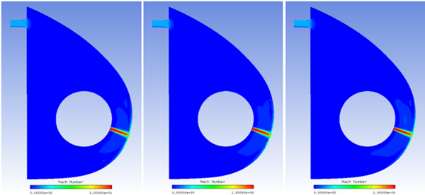
Figure 7.59: Initial Internal Airflow Results: Surface Pressure (Left: CFX; Middle: Fluent; Right: FENSAP)
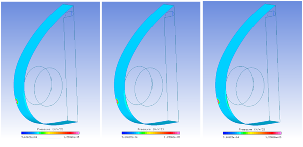
Figure 7.60: Initial Internal Airflow Results: Surface Shear Stress (Left: CFX; Middle: Fluent; Right: FENSAP)
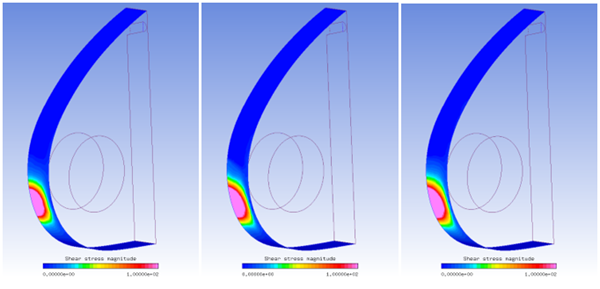
Figure 7.61: Initial Internal Airflow Results: Surface Heat-flux (Left: CFX; Middle: Fluent; Right: FENSAP)
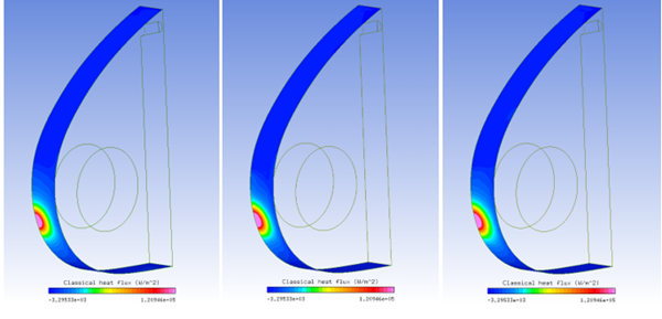
Note: To appropriately compare the results of this CHT anti-icing simulation using CFX with the kw-sst turbulence model, another CHT anti-icing simulation using FENSAP with its own kw-sst turbulence model was conducted. Piccolo Tube Operating in the Wet Air Regime (Anti-Icing) uses the Spalart-Allmaras turbulence model and therefore its results are not suitable to make proper comparisons. Results and comparisons of all kw-sst cases are presented throughout this tutorial and show that CFX and FENSAP/Fluent produce similar CHT results.
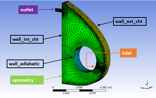
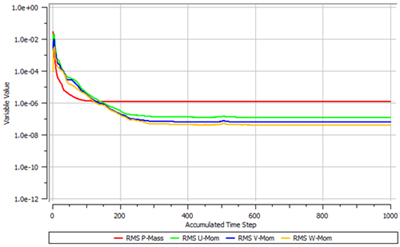
Open the PICCOLO_CFX project with FENSAP-ICE. Use → menu or the new run icon to create a new DROP3D run. Name this run
DROP3D_ext_CFX.Right-click the grid icon and select . Navigate to the folder,
INITIAL-AIR, and select,CFX- piccolo-ext_001.res. Then press and a new Grid converter window appears. Accept the default options and click or .The Grid converter will now execute. When done, click . The mesh and airflow solution in FENSAP format of CFX res file will now appear in the grid and airsol input sections to the left of the config icon.
Double-click the DROP3D_ext_CFX config icon to edit the input parameters.
Go to the Conditions panel and verify that the Reference conditions and Droplet initial solution contains the information shown as below.
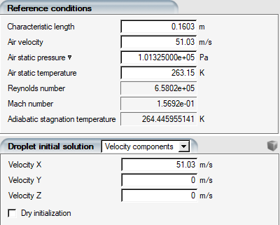
Note: When importing the CFX .res file into FENSAP-ICE, the converter takes the CFX air properties at the Inlet boundary conditions as reference conditions. Therefore, it is recommended that you verify that these reference conditions are appropriate to the physical problem that you are solving.
In the Conditions panel, set the following Droplet reference conditions.
Liquid Water Content 1g/m3Droplet diameter 20micronsWater density 1000kg/m3Go to the Boundaries panel. Select the BC_1000 (Inlet) boundary surface and click .
Go to the Solver panel. Set the CFL number to
20and the Maximum number of time steps to300. Click the button. Start the calculation on4or more CPUs if possible.The following figures show the computed liquid water content and collection efficiency and compare these results against a DROP3D solution obtained from a FENSAP/Fluent kw-sst airflow.
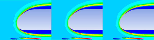
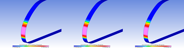
The goal of this step is not to provide an initial ice shape, but rather to establish a water film on the outer surface of the solid as an initial condition for the wet CHT run.
Create a new ICE3D run and name it
ICE3D_ext_CFX.Drag & drop the config icon of DROP3D_ext_CFX onto the config icon of this new run. This operation automatically links the air and droplet solutions, the grid of the external domain and the reference conditions into the ICE3D_ext_CFX run.
Double-click the config icon to edit the input parameters.
Go to the Model panel. Change the Icing model to and select in Heat flux type.
Go to the Conditions panel. Set the Recovery factor to
0.9.Go to the Solver panel. Keep the Automatic time step option enabled and change the Total time of ice accretion to
30seconds.Run the calculation on
4or more CPUs if possible.
Create a new CHT3D run and name it
CHT3D_wet_CFX. The CHT configuration window will appear to prompt for the type of CHT simulation desired. Select in the Problem type pull-down menu, then choose . Select in the Flow Solver (External) and (Internal) settings. Press the button to continue with the setup. A tree of coupled CFX, ICE3D and C3D runs will appear in the run window.Right-click the grid icon of fluid_ext and select . Navigate to the INITIAL-AIR folder and select the CFX-piccolo-ext_001.res file. Then press . Select to import the settings again. A new Grid converter window.
Double-click the config icon of the fluid_ext run to edit the input parameters. In the CFX configuration window, do the following:
Set the Number of iterations to
50;Set the RMS Convergence criteria to
1e-12;Set the correct path to the CFX executable;
Set the launch Parameters to
“-batch $EXTRA_CFX_ARGS -par-local -part $NCPU”.Click to close the CFX configuration window.
Drag & drop the config icon from ICE3D_ext_CFX onto the config icon of the ice_ext run in CHT3D_wet_CFX.
Right -click the grid icon of fluid_int and select . Navigate to the INITIAL-AIR folder and select the CFX-piccolo-int_001.res file. Press . A new Grid converter window appears. Accept the default options and click or . Once the grid and solution conversions are complete, click to close this window.
Note: When the Reference parameters table appears in the Grid converter window, double-check and make sure that the Reference velocity magnitude and the X, Y, and Z-velocity component directions are correct. For this case, the following values should be used:
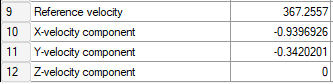
Double-click the config icon of the fluid_int run to edit the input parameters. In the CFX configuration window, do the following:
Set the Number of iterations to
50;Set the RMS Convergence criteria to
1e-12;Set the correct path to the CFX executable;
Set the launch Parameters to
“-batch
          $EXTRA_CFX_ARGS -par-local -part $NCPU”
. Click to close the CFX configuration window.
To set up the solid run in CHT3D_wet_CFX, double-click the grid_material icon and select the file piccolo_solid provided under the tutorials subdirectory CHT.
Go to the Settings panel. Set the Temperature value to
300K (26.85 °C). This will be the initial temperature throughout the solid domain.Go to the Properties panel. Click the button to change the material name from default to duralumin. Specify the following characteristics for the material:
Density 2787kg/m3Conductivity 164W/m/KEnthalpy 241060J/kgGo to the Materials panel. Since duralumin is the only material in the solid domain, the label MAT_0 will be automatically assigned to it.
Go to the Boundaries panel. Define the boundary conditions of the outer surfaces of the solid as follows:
BC_2001: Default settings (Thermal BC definition set to Nothing)
BC_2002: Default settings (Thermal BC definition set to Nothing)
BC_2004: Default settings (Thermal BC definition set to Nothing)
BC_2005: Set Thermal BC definition to Flux Type and Heat flux to
0W/m2BC_2006: Set Thermal BC definition to Flux Type and Heat flux to
0W/m2BC_2007: Set Thermal BC definition to Flux Type and Heat flux to
0W/m2BC_4100: Set Thermal BC definition to Flux Type and Heat flux to
0W/m2BC_4300: Set Thermal BC definition to Flux Type and Heat flux to
0W/m2Note: CHT3D will automatically update the boundary conditions on BC_2001, BC_2002, and BC_2004 during the simulation.
Go to the Solver panel. Select from the Time step drop-down menu. Set the Time step value to
0.1seconds and the Total time to5seconds. At each CHT3D iteration, heat conduction will be computed for 5 seconds. Close and save this configuration.Double-click the main config icon of CHT3D_wet_CFX to set up the links between the solid and fluid domains.
Figure 7.64: The 3 Computational Domains: Blue (External), Red (Internal), Green (Solid). Right: Stagnation Point

Go to the Parameters panel. Set the Number of CHT iterations (loops) to
30and Solution output every0seconds (default value).Choose the option in the Flow solver mode pull-down menu for both external and internal flow.
Go to the Interfaces panel. There are three fluid/solid interfaces in the computational domain. CHT3D will automatically exchange the boundary conditions between these three interfaces. Set up the interfaces as follows:
For External to Solid: There is only one interface between the external domain and the solid. Set the interface boundaries as follows:
External fluid grid: 2000: wall_cht
Solid grid: 2001
For Solid to Internal: There are two interfaces between the solid and the internal domain. Set the first interface as follows:
Solid grid: 2002
Internal fluid grid: 2001: wall_ext_cht
Then click
next to
Interface label of Solid to Internal to add the
third interface and set it as follows:Solid grid: 2004
Internal fluid grid: 2002: wall_int_cht
Go to the Temperatures panel. Set the External Surface recovery temperature to
264.316K (-8.834 °C). Set the Internal adiabatic stagnation temperature to402.52K (129.37 °C).Note: The value of the External Surface recovery temperature is computed by applying a recovery factor of 0.9 on the total temperature of the external airflow. The value of the Internal adiabatic stagnation temperature is the total air temperature at the jet hole of the internal domain. Both values are used as reference temperatures, for the external and internal domains respectively, during a CHT simulation.
Close and save the configuration.
Right-click the main config icon of CHT3D_wet_CFX, then select the Run option in the menu to launch the CHT3D calculation. Use
4or more CPUs for all solvers if possible, and launch the calculation.This simulation takes a substantial amount of time to complete.
Figure 7.65: Convergence History of the Maximum Solid Wall Temperatures (Left: CFX; Middle: Fluent; Right: FENSAP)
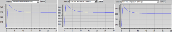
Figure 7.66: Convergence History of the Minimum (Right) Solid Wall Temperatures (Left: CFX; Middle: Fluent; Right: FENSAP)
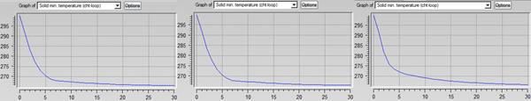
Figure 7.68: Water Film Thickness on the External Surface (ICE3D) (Left: CFX; Middle: Fluent; Right: FENSAP)
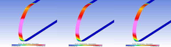
Figure 7.69: Instantaneous Ice Growth on the External Surface (ICE3D) (Left: CFX; Middle: Fluent; Right: FENSAP)
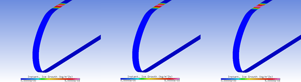
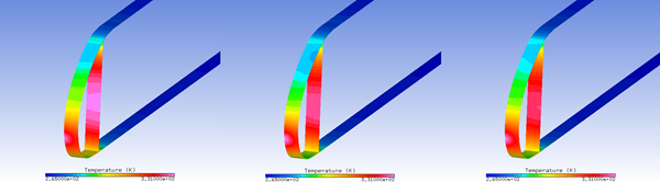
If ice is expected to form during a CHT simulation (due to insufficient heating or as designed), you should impose a sand-grain roughness over the contaminated surfaces. In this manner, the shape and the thickness of the ice will be more accurately represented over these zones. In CHT3D, this is done by enabling the surface roughness option in the main configuration window. Since roughness changes the turbulence and velocity profiles which consequently change the heat fluxes and shear stresses, the full Navier-Stokes equation should be solved on the external domain during CHT iterations. Roughness will be applied only in regions where the instantaneous ice growth rate is non-zero, while the rest of the surface remains smooth.
Create a new CHT3D run and name it
CHT3D_wet_CFX_with_roughness. The CHT configuration window will appear to prompt for the type of CHT simulation desired. Select in the Problem type pull-down menu, then choose . Select in the Flow Solver (External) and (Internal) settings. Click to continue with the setup. A tree of coupled CFX, ICE3D and C3D runs will appear in the run window.Drag & drop the config icon of CHT3D_wet_CFX onto the config icon of the main CHT3D_wet_CFX_with_roughness run, and click the button. This will copy all the necessary input files and parameters for the current simulation.
Double-click the main config icon of CHT3D_wet_CFX_with_Roughness to open the configuration window.
Go to the Parameters panel. Set the Number of CHT iterations to
30and Solution output every0iterations (default value).Choose the option in the Flow solver mode – external pull-down menu.
Set the Ice roughness to and enter
0.0005meters (default value). Choose the option in the Flow solver mode – internal pull-down menu.Click and the current run settings.
Right-click the main config icon of CHT3D_wet_CFX_with_Roughness. Select the Run option in the menu to launch the CHT3D calculation. Use
4or more CPUs for all solvers if possible.Figure 7.71: Water Film Thickness on the External Surface (ICE3D) (Left: CFX; Middle: Fluent; Right: FENSAP)
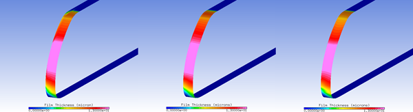
Figure 7.72: Instantaneous Ice Growth on the External Surface (ICE3D) (Left: CFX; Middle: Fluent; Right: FENSAP)
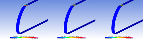
From the heat transfer point of view on the protected zone, there is not much difference between this case and the previous one. The actual difference will be visible when the ice shape after CHT is computed in the next sections.
After the CHT computation is complete, the rate at which ice will accrete can be assessed by looking at the Instantaneous Ice Growth data field in the ICE3D solution file swimsol. However, the amount of ice can be visualized by performing a post-CHT ICE3D simulation.
Create a new ICE3D run and name it
ICE3D_post_CHT_CFX.Drag & drop the config icon of the ice_ext section of the CHT3D_wet_CFX simulation onto this new ICE3D run. This operation automatically links the air and droplet solutions, heat fluxes, grid of the external domain and the reference conditions into the ICE3D_post_CHT_CFX.
Double-click the config icon to edit the input parameters.
Go to the Solver panel. Keep the option enabled and change the Total time of ice accretion to
2400seconds.Go to the Out panel. Set the Time between solution output to
2400seconds. This will only output and write the final solution.Run the calculation. Use
4or more CPUs if possible.
Figure 7.73: Residual Ice Shape Accreted for 2400 Seconds with the Hot Air IPS Turned On (Left: CFX; Middle: Fluent; Right: FENSAP)
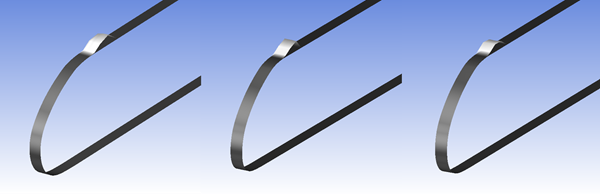
After the CHT computation is done, the rate at which ice will accrete can be assessed by looking at the Instantaneous Ice Growth data field in the ICE3D solution file swimsol. However, the amount of ice can be visualized by performing a post-CHT ICE3D simulation.
Create a new ICE3D run and name it
ICE3D_post_CHT_CFX_with_roughness.Drag & drop the config icon of the ice_ext section of the CHT3D_wet_CFX_with_roughness simulation onto this new ICE3D run. This operation automatically links the air and droplet solutions, heat fluxes, grid of the external domain and the reference conditions into the ICE3D_post_CHT_CFX_with_roughness.
Double-click the config icon to edit the input parameters.
Go to the Solver panel. Keep the Automatic time step option enabled and change the Total time of ice accretion to
2400seconds.In the Out panel, set the Time between solution output to
2400seconds. This will only output and write the final solution. Select from the drop-down menu of the Generate displaced grid option to get the displaced-iced grid for additional flow computations (optional).Run the calculation. Use
4or more CPUs if possible.Note: To compare the ice shapes obtained without and with roughness in CHT, first load the ice shape of ICE3D_post_CHT_CFX. Go back to the project window and right-click the swimsol icon of the ICE3D_post_CHT_CFX_with_roughness run. Choose and load it in a new window. Next, click the button of the current run and . The two grids should be loaded with the ice shapes on them. Split the screen to put the data sets on either side of the view.
Figure 7.74: Residual Ice Shape Accreted for 2400 Seconds With the Hot Air Ips Turned On, With Roughness (Left: CFX; Middle: Fluent; Right: FENSAP)
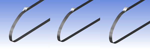
To view the displaced external flow grid, right-click the grid_disp icon of the ICE3D_post_CHT_CFX_with_roughness run and select .
Note: The displaced grid can be used for performance analysis to see the adverse effects of the residual ridge ice.
This tutorial illustrates the procedure for computing Conjugate Heat Transfer (CHT) through the metal skin of the leading edge of a wing heated by electro-thermal pads. The CHT analysis is performed in wet air.
Create a new project using → menu or the New project icon and name it
DEICER. Select the metric unit system.Create a new FENSAP run using → menu or the new run icon and name it
FENSAP_ext.Double-click the grid icon and select the grid file deicer_ext provided in the tutorials subdirectory DEICER. The hexahedral mesh is composed of 66,080 elements and 133,318 nodes.
Double-click the config icon of the FENSAP_ext run to edit the input parameters for the external flow calculation.
Go to the Model panel and select the Navier-Stokes option for the Momentum equations and Full PDE for the Energy equation.
Select the Spalart-Allmaras turbulence model and set the Eddy/laminar viscosity ratio to a very low value,
1e-5.Select the Specified sand-grain roughness option in the Surface roughness section and set the roughness height to
0.0005m.Note: As opposed to anti-icing runs, deicing runs do contain ice formation, therefore roughness should be enabled in the flow solver to account for the iced surface roughness effects on heat fluxes.
Go to the Conditions panel and set the following Reference conditions:
Characteristic length 0.9144mAir velocity 44.704m/sAir static pressure 101325PaAir static temperature 266.483K (-6.667°C)In order to reduce the amount of time required to run this tutorial, a converged external flow solution can be found in the tutorials subdirectory ../workshop_input_files/Input_Grid/DEICER. Change the Initial solution option from Velocity components to Solution restart and select the solution file deicer_ext_restart.
Note: To start this calculation without a restart solution file, select the Velocity components option from the Initial solution submenu and set the Velocity X to
44.704m/s. The remaining velocity components should be set to0m/s.Go to the Boundaries panel, select the inlet boundary BC_1001 and choose Supersonic or far-field in Type section. Click the button to set the Inlet conditions. Assign Velocity X to
44.704m/s and the remaining velocity components to0m/s.Select the wall boundary BC_2001 that corresponds to the protected region on the leading edge, and set its Temperature value to
288K (14.85°C).Note: Temperature must be imposed on the leading edge in order to compute an initial nonzero heat flux to start the CHT calculation. This temperature is automatically updated during the CHT3D loop.
Repeat the same procedure for the wall boundaries BC_2008 and BC_2009, which are the two unprotected sections of the wing.
Go to the Solver panel. Choose the Steady option in the Time integration section. Set the CFL number value to
100and Maximum number of time steps value to1. Uncheck the Use variable relaxation option. In the Artificial viscosity option, select Streamline upwind and set the Cross-wind dissipation value to1e-09. FENSAP will restart from the restart solution file, deicer_ext_restart, and write all the output files required for the CHT3D simulation.Note: To start this calculation without a restart solution file, set the Maximum number of time steps to
1200.In the Out panel, set the solution write frequency to every
20iterations to be able to visualize convergence of total heat flux in the Graphs panel during execution.Click the button at the bottom of the window to go to the execution environment and run this restart calculation on
4processors. The solution look like the one shown in the following figure.
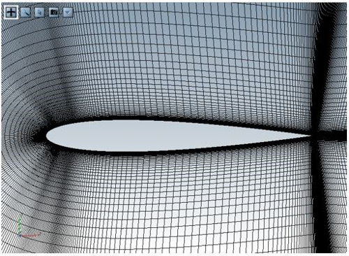
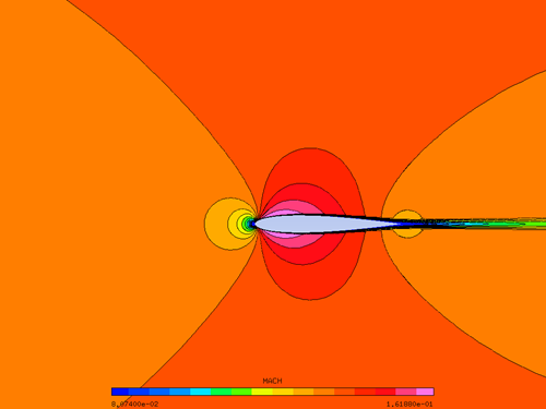
Create a new DROP3D run using the → menu or the new run icon and name it
DROP3D_ext.Drag & drop the config icon of the FENSAP_ext run onto the config icon of the new DROP3D run.
Double-click the DROP3D_ext config icon to edit the input parameters.
Go to the Conditions panel and set the following Droplet reference conditions:
Liquid Water Content 0.78g/m3Droplet Diameter 20micronsTo reduce the amount of time required to run this tutorial, a converged droplet solution can be found in the tutorials subdirectory DEICER. In the Droplets initial solution section, change the Velocity components option to Solution restart and select the solution file deicer_droplet_restart.
Note: To start this calculation without a restart solution file, select the Velocity components option from the Droplets initial solution submenu and set the Velocity X component to
44.704m/s. The remaining velocity components should be set to0m/s.Go to the Boundaries panel, select the Inlet boundary BC_1001 and click the Import reference conditions button.
Go to the Solver panel, set the Maximum number of time steps to
1.Note: To start this calculation without a restart solution file, keep the default CFL number and Maximum number of time steps as
20and120, respectively.Click the button at the bottom of the window to go to the execution environment and run this restart calculation on
4processors. The collection efficiency distribution should look very similar to the one shown in the following figure. If running without a restart, check the Total Beta and Change in total Beta graphs to follow the convergence process.
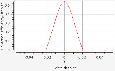
Create a new CHT3D run using the → menu or the new run icon and name it
CHT3D_deicer.The CHT configuration window opens and prompts for the type of CHT simulation:
Select Electro-thermal (1 fluids, 1 solid) in the Problem type pull-down menu.
Select Wet air
Select the De-icing option in the Icing mode pull-down menu.
Click the button to continue with the set-up. A hierarchy of coupled FENSAP, ICE3D and C3D runs will appear in the run window.
To configure the external flow run, drag & drop the configuration icon of the previous FENSAP_ext run onto the configuration icon of the fluid_ext run in CHT3D_deicer. The convective heat transfer will be based on the heat transfer coefficients computed during the initial FENSAP run.
To configure the ice accretion run, drag & drop the config icon of the previous DROP3D_ext run onto the configuration icon of the ice_ext run.
Double-click the config icon of the ice_ext run to configure the parameters. In the Model panel, select Classical for the Heat flux type under Icing model; in the Conditions panel, set the Recovery factor value to
0.9, then close the configuration panel and save the changes.To configure the solid run in CHT3D_deicer, double-click the grid icon and select the file deicer_solid provided in the tutorial subdirectory ../workshop_input_files/Input_Grid/DEICER.
Double-click the config icon of the solid run to edit the input parameters for heat conduction.
Go to the Settings panel. Set Temperature to
264.15K (-9°C). This is the initial temperature throughout the solid domain.Go to the Properties panel. Define four materials with the following characteristics:
Erosion shield
Density 8025.25kg/m3Conductivity 16.26W/m/KEnthalpy 137234.93J/kgElastomer
Density 1383.9552kg/m3Conductivity 0.2561W/m/KEnthalpy 343087.33J/kgFiberglass/epoxy
Density 1794kg/m3Conductivity 0.294W/m/KEnthalpy 428859.16J/kgSilicone foam
Density 648.75kg/m3Conductivity 0.121W/m/KEnthalpy 308778.6J/kg
Go to the Materials panel. Select the Material type for each region of the grid:
MAT 1 = Erosion shield
MAT 2 = Elastomer
MAT 3 = Fiber glass/epoxy
MAT 4 = Silicone foam
Go to the Boundaries panel. Define the boundary conditions of the outer surfaces of the solid as follows:
BC_2001: Default settings (Thermal BC definition set to Nothing)
BC_2002: Select Mixed type for Thermal BC definition and set the Temperature to
266.48333K (-6.66667°C) and the Heat coefficient to100W/m2/KBC_4000: Default settings (Thermal BC definition set to Nothing)
BC_4300: Default settings (Thermal BC definition set to Nothing)
BC_6001: Set the Heat flux to
0W/m2/KBC_6002: Set the Heat flux to
0W/m2/KBC_6003: Set the Heat flux to
0W/m2/KBC_6004: Set the Heat flux to
0W/m2/KBC_6005: Set the Heat flux to
0W/m2/KBC_6006: Set the Heat flux to
0W/m2/KBC_6007: Set the Heat flux to
0W/m2/KNote: CHT3D will automatically apply interface boundary conditions on BC_2001 during the simulation.
Go to the Cycles panel. The de-icing simulation consists of 5 cycles of activation and de-activation of heater pads. Each cycle lasts 120 seconds and has the following properties:
BC Type Start at (s) Duration (s) Heat Flux (W/m2) Heater 1 (BC_6001) 0 120 7750 Heater 2 (BC_6002) 100 10 15500 Heater 3 (BC_6003) 100 10 15500 Heater 4 (BC_6004) 110 10 12400 Heater 5 (BC_6005) 110 10 12400 Heater 6 (BC_6006) 110 10 12400 Heater 7 (BC_6007) 110 10 12400 To create and configure one single de-icing cycle from the above table, inside the Cycles submenu, click the
button next to Cycle to create a new cycle, the
default name is Cycle
A. Set the Duration of Cycle
A to 120seconds and press Enter.Note: When a new cycle is created, a default Duration of 10 seconds will be assigned and a heater from the drop box of BC, in Current selection, will be pre-selected as the default heater.
Under Current selection, do the following:
Select Heater 1 from the drop box of BC. Change the unit of Start from % to s and set its value to
0. Change the unit of Duration from % to s and set its value to120seconds. Make sure Constant is selected in the drop box of Heat Flux and set the heat flux value to7750W/m2. This configures the properties of Heater 1 in the table above.Click the
button above the Current selection section to
(create) define another heater for Cycle A. Select Heater
2 from the drop box of BC. Refer to the properties of
Heater 2 in the table above and repeat the same steps of
Heater 1 to continue to set up Heater 2.Repeat the same steps to define and to set up the rest of the heaters in the table above.
The figure below shows the final configuration of one de-icing cycle.
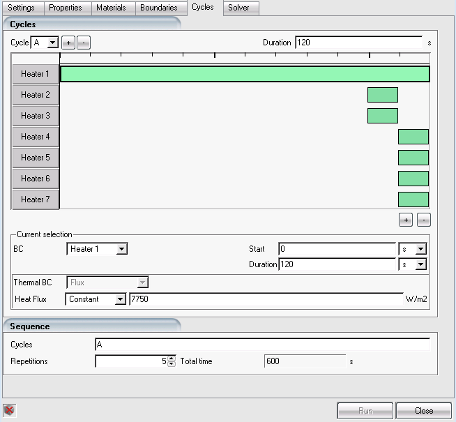
Note: The green bars in the figure above illustrate how heaters behave within a de-icing cycle. Clicking on each bar will update the properties in the Current selection for the selected heater.
In the Sequence submenu, set Cycles to A and the Repetitions to
5as Cycle A is repeated 5 times. In this manner, the Total time of the de-icing simulation is 600 seconds.Click to save the configuration file and close the window.
Double-click the main config icon of the CHT3D_deicer run to define the common interfaces between the solid and fluid domains.
Go to the Parameters panel. Use the table shown below to configure the parameters of the Run parameters submenu.
Time stepping Automatic Maximum time step 0.5seconds - This is the de-icing simulation time step.Unsteady total time 600seconds - This is the total de-icing simulation time.Icing sub-iterations 1000Iter. Per time step 10- This is the number of CHT loops per time step.Solution output every 1seconds - To save all solutions of de-icing simulation every second.Go to the Interfaces panel. There is only one fluid/solid interface in the computational domain. CHT3D will automatically exchange the boundary conditions between these two interfaces. Set up the interface as follows:
External fluid: 2001
Solid: 2001
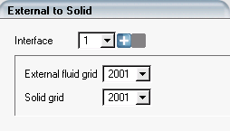
Click the button to save the configuration and close the window.
To launch CHT3D, right-click the main config icon of CHT3D_deicer, then select the option in the menu to launch the CHT3D calculation. In the execution environment, set the number of CPUs to
4for ICE3D and C3D.Note: The simulation progress can be monitored in the Log and Graphs panels.
The following graph shows the history of the maximum temperature of the solid domain throughout the simulation.
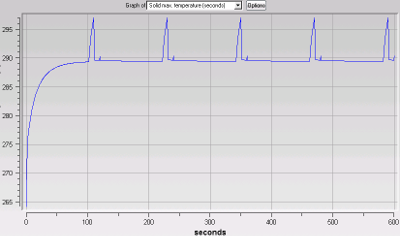
The following graph shows the history of the temperature at three locations on the surface and compares them to experimental data.
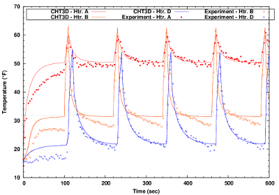
The following figures show snapshots of the leading edge solid temperature distribution as well as the ice layer at four distinct times.
Figure 7.80: Residual Ice Shape and Solid Temperature at (a) 100, (b) 110, (c) 120 and (d) 220 Seconds
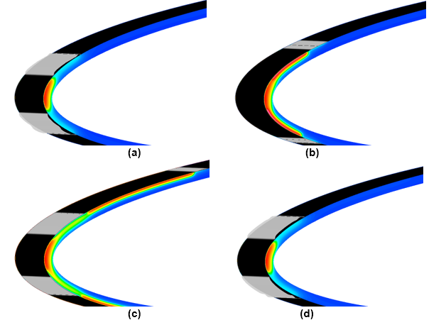
This tutorial illustrates the procedure for computing Conjugate Heat Transfer (CHT) through the metal skin of the leading edge of a wing heated by electro-thermal pads. The CHT analysis is performed in wet air.
Using the FENSAP-ICE interface, create a new project using → menu or the New project icon and name it as
DEICER_FLUENT. Select the metric unit system.Go to the project folder, DEICER_FLUENT, and create a new sub folder INITIAL-AIR. Copy the provided Fluent case file, FLUENT-deicer_ext.cas.h5, from the tutorials subdirectory DEICER to this new folder and launch Fluent.
Note: In Windows, Fluent can be launched by going to Start → All Programs → ANSYS 2024 R2 → Fluid Dynamics → Fluent 2024 R2.
In the Fluent Launcher window, select Dimension as 3D, pick Double Precision under Options, and assign
2to4CPUs under Solver Processes. Click Show More Options. Under General Options, set your Working Directory to the INITIAL-AIR directory. Press to close the Fluent Launcher.Note: Select Serial under Processing Options to run the simulation using a single processor or CPU if multiple processes are not available.
Read the case file by going to the → → menu and browse to and select the Fluent case file, FLUENT-deicer_ext.cas.h5, located inside the sub folder INITIAL-AIR.
From the top bar menu, select Physics. Make sure the Solver is set to Pressure-Based, Absolute, and Steady. Click the Operating Conditions. Set the Operating Pressure to
0Pa. Press to close the Operation Conditions window.Expand the Setup → Material → Fluid from the side tree menu. Double-click air and modify its properties. The table below describes the air properties to be imposed in this simulation.
Density Ideal-gas Cp 1004.688J/kg-KThermal Conductivity 0.23499201E-01W/m-KViscosity 1.68424887e-05kg/m-sMolecular Weight 28.966kg/kgmolClick the button and this window to save the new air properties.
Note: Thermal conductivity and viscosity are computed from these equations which are presented in the FENSAP-ICE User Manual and shown below:
In these equations, T∞ refers to the ambient air static temperature, and C1, Tref and µref are equal to 0.00216176 W/m/K3/2, 288 K and 17.9*10-6 Pa s respectively.
Expand and double-click Setup → Models → Viscous from the side tree menu. Select the k-omega (2 eqn) option in the opened Viscous Model interface and then select k-omega Model → SST. Make sure that Viscous Heating and Production Limiter are activated in the Options section. In the Model Constants section, drag the scroll bar down and set Energy Prandtl Number and Wall Prandtl Number values to
0.9. Click to close this menu.Expand and double-click Setup → Models → Energy from the side tree menu. Ensure that Energy is turned on.
Expand and double-click Setup → Boundary Conditions from the side tree menu. In the Task Page, click Periodic Conditions and set the Flow Direction vector (X, Y, Z) to (
0,0,1). Then close this window.In the Task Page → Boundary Conditions list, double-click pressure-far-field-4 and configure the below:
Momentum panel
Gauge Pressure 101325PaMach Number 0.1366048X, Y and Z-Components of Flow Direction 1,0,0Turbulence Specification Method Intensity and Viscosity Ratio Turbulence Intensity 0.08%Turbulent Viscosity Ratio 1e-5Thermal panel
Temperature 266.483KDouble-click wall-5 and configure the Momentum panel as follows
Wall Motion Stationary Wall Shear Condition No Slip Wall Roughness (Roughness Models) High Roughness (Icing) Specified Roughness Roughness Height (m) 0.0005Roughness Constant 0.5Thermal panel
Temperature 288K
Expand and double-click Setup → Reference Values from the side tree menu. In the Task Page window, use the Compute from drop-down menu to select pressure-far-field-4.
Expand and double-click Solution → Methods from the side tree menu. Set Pressure-Velocity Coupling to Coupled. In the Spatial Discretization section, set the Gradient to Green-Gauss Node Based and the remaining settings to Second Order or Second Order Upwind. Enable Pseudo Transient and High Order Term Relaxation.
Expand and double-click Solution → Monitors → Residual from the side tree menu. In the Residual Monitors window, make sure that the Print to Console and the Plot are enabled. Disable all check box below the Convergence column. Close this window once this is done.
Expand and double-click Solution → Initialization from the side tree menu. In the Task Page window, select Hybrid Initialization under Initialization Methods. Click the button to initialize the computational domain.
Expand and double-click Solution → Run Calculation from the side tree menu. Under the Pseudo Transient Options, set the Time Step Method to Automatic and the Timescale Factor to
1. Enter3000as the total Number of Iterations and click Calculate to start the simulation.Once the simulation is complete, save the new Fluent solutions in → → . Name this simulation as
FLUENT-deicer_ext.cas.h5/dat.h5.
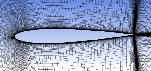


Go back to the FENSAP-ICE project folder DEICER_FLUENT and create a new DROP3D run using the → menu or the new run icon. Name this run
DROP3D_ext_FLUENT.Right-click the grid icon and select the Define option. Navigate to the folder INITIAL-AIR and select FLUENT-deicer_ext.cas.h5. Press Open and a new Grid converter window appears. Accept the default options and click or Next. Once the grid and solution conversions are completed, click the Finish button to close this window.
Double-click the DROP3D_ext_FLUENT config icon to edit the input parameters.
Go to the Conditions panel and set the following Droplet reference conditions:
Liquid Water Content 0.78g/m3Droplet diameter 20micronsTo reduce the amount of time required to run this tutorial, a converged droplet solution can be found in the tutorials subdirectory DEICER. In the Droplets initial solution section, change the Velocity components option to Solution restart and select the solution file FLUENT-deicer_droplet_restart.
Note: To start this calculation without a restart solution file, select the Velocity components option from the Droplets initial solution submenu and set the Velocity X component to
44.704m/s. The remaining velocity components should be set to0m/s.Go to the Boundaries panel, select the Inlet boundary BC_1001 and click the Import reference conditions button. Make sure the Velocity X component is
44.704m/s and the remaining velocity components are set to0m/s.Go to the Solver panel, set the Maximum number of time steps to
1.Note: To start this calculation without a restart solution file, set the CFL number to
20and the Maximum number of time steps to800. Double-click the Advanced solver settings bar, change the Convergence level to1e-10and the Change in total beta to1e-12.Click the button at the bottom of the window to go to the execution environment and run this restart calculation on
4processors. The collection efficiency distribution should be very similar to the one shown in the following figure.
Inside the DEICER_FLUENT project, create a new CHT3D run using the → menu or the new run icon. Name this run
CHT3D_deicer_FLUENT.The CHT configuration window opens and prompts for the type of CHT simulation to conduct:
Select Electro-thermal (1 fluids, 1 solid) in the Problem type pull-down menu.
Select Wet air
Select the De-icing option in the Icing mode pull-down menu.
Click the button to continue with the set-up. A hierarchy of coupled FENSAP, ICE3D and C3D runs will appear in the run window.
Note: In FENSAP-ICE 2024 R2, the de-icing mode of CHT3D doesn’t naturally support Fluent as the external flow run. CHT3D does not directly support a hierarchy of coupled Fluent, ICE3D and C3D runs. A work around is shown in the next step.
To configure the external flow run, do the following:
Drag & drop the grid and airsol icons of previous the DROP3D_ext_FLUENT run onto the grid and airsol icons of fluid_ext respectively.
Right-click the heatflux icon of fluid_ext and select Define. Navigate to the INITIAL-AIR folder and select FLUENT-deicer_ext.hflux;
Right-click the forces icon of fluid_ext and select Define. Navigate to the INITIAL-AIR folder and select FLUENT-deicer_ext.surface;
Double-click the config icon of fluid_ext and configure as follows:
Model panel
Select Navier-Stokes from the drop box of the Momentum equations and K-omega SST from the drop box of the Turbulence model. Set Eddy/Laminar viscosity ratio value to
1e-5and Turbulence intensity to0.0008.Conditions panel
Characteristic length 0.9144mAir velocity 44.704m/sAir static pressure 101325PaAir static temperature 266.483K (-6.667°C)Boundaries panel
Select the inlet boundary pressure-far-field-4 and specify Supersonic or far-field in the Type dropdown. Set the Pressure to
101325Pa, the Temperature to266.483K, and the Velocity components (X, Y, Z) to (44.704,0,0) m/s. Press Ctrl + left-click to select wall-5, wall-6, and wall-7 in the Boundary Conditions menu. Set No-slip in Surface type with a Temperature of288K.Solver panel
Set the Cross-wind dissipation to
1e-09under Artificial viscosity.
Close the configure panel and save the changes.
To configure the ice accretion run, drag & drop the config icon of the previous DROP3D_ext_FLUENT run onto the config icon of the ice_ext run.
Double-click the config icon of the ice_ext run to configure the parameters. In the Model panel, select Classical for the Heat flux type under Icing model. In the Conditions panel, set the Recovery factor to
0.9, then close the configuration panel and save the changes.To configure the solid run in CHT3D_deicer, double-click the grid icon and select the file deicer_solid provided in the tutorial subdirectory DEICER.
Double-click the config icon of the solid run to edit the input parameters for heat conduction.
Go to the Settings panel. Set Temperature to
264.15K (-9°C). This is the initial temperature throughout the solid domain.Go to the Properties panel. Define four materials with the following characteristics:
Erosion shield
Density 8025.25kg/m3Conductivity 16.26W/m/KEnthalpy 137234.93J/kgElastomer
Density 1383.9552kg/m3Conductivity 0.2561W/m/KEnthalpy 343087.33J/kgFiberglass/epoxy
Density 1794kg/m3Conductivity 0.294W/m/KEnthalpy 428859.16J/kgSilicone foam
Density 648.75kg/m3Conductivity 0.121W/m/KEnthalpy 308778.6J/kg
Go to the Materials panel. Select the Material type for each region of the grid:
MAT 1 = Erosion shield
MAT 2 = Elastomer
MAT 3 = Fiber glass/epoxy
MAT 4 = Silicone foam
Go to the Boundaries panel. Define the boundary conditions of the outer surfaces of the solid as follows:
BC_2001: Default settings (Thermal BC definition set to Nothing)
BC_2002: Select Mixed type for Thermal BC definition and set the Temperature to
266.48333K (-6.66667°C) and the Heat coefficient to100W/m2/KBC_4000: Default settings (Thermal BC definition set to Nothing)
BC_4300: Default settings (Thermal BC definition set to Nothing)
BC_6001: Set the Heat flux to
0W/m2/KBC_6002: Set the Heat flux to
0W/m2/KBC_6003: Set the Heat flux to
0W/m2/KBC_6004: Set the Heat flux to
0W/m2/KBC_6005: Set the Heat flux to
0W/m2/KBC_6006: Set the Heat flux to
0W/m2/KBC_6007: Set the Heat flux to
0W/m2/K
CHT3D will automatically apply interface boundary conditions on BC_2001 during the simulation.
Go to the Cycles panel. The de-icing simulation consists of 5 cycles of activation and de-activation of heater pads. Each cycle lasts 120 seconds and has the following properties:
BC Type Start at (s) Duration (s) Heat Flux (W/m2) Heater 1 (BC_6001) 0 120 7750 Heater 2 (BC_6002) 100 10 15500 Heater 3 (BC_6003) 100 10 15500 Heater 4 (BC_6004) 110 10 12400 Heater 5 (BC_6005) 110 10 12400 Heater 6 (BC_6006) 110 10 12400 Heater 7 (BC_6007) 110 10 12400 To create and configure one single de-icing cycle from the above table, inside the Cycles submenu, click the
button next to Cycle to create a new cycle, the
default name is Cycle
A. Set the Duration of Cycle
A to 120seconds and press Enter.Note: When a new cycle is created, a default Duration of 10 seconds will be assigned and a heater from the BC dropdown, in Current selection, will be pre-selected as the default heater.
Under Current selection, do the following:
Select Heater 1 from the BC dropdown. Change the unit of Start from % to s and set its value to
0. Change the unit of Duration from % to s and set its value to120seconds. Make sure Constant is selected in the Heat Flux dropdown and set the heat flux value to7750W/m2. This configures the properties of Heater 1 in the table above.Click the
button above the Current selection section to
(create) define another heater for Cycle A. Select Heater
2 from the BC dropdown. Refer to the properties of
Heater 2 in the table above and repeat the same steps of
Heater 1 to continue to set up Heater 2. Repeat the same steps to define and to set up the rest of the heaters in the table above.
The figure below shows the final configuration of one de-icing cycle.

Note: The green bars in the figure above illustrate how heaters behave within a de-icing cycle. Clicking on each bar will update the properties in the Current selection for the selected heater.
In the Sequence submenu, set Cycles to A and the Repetitions to
5as Cycle A is repeated 5 times. In this manner, the Total time of the de-icing simulation is 600 seconds.Click to save the configuration file and close the window.
Double-click the main config icon of CHT3D_deicer_FLUENT to define the common interfaces between the solid and fluid domains.
Go to the Parameters panel. Use the table shown below to configure the parameters of the Run parameters submenu.
Time stepping Automatic - Maximum time step 0.5secondsThis is the de-icing simulation time step. Unsteady total time 600secondsThis is the total de-icing simulation time. Icing sub-iterations 1000- Iter. Per time step 10This is the number of CHT loops per time step. Solution output every 1secondsTo save all solutions of de-icing simulation every second. Go to the Interfaces panel. There is only one fluid/solid interface in the computational domain. CHT3D will automatically exchange the boundary conditions between these two interfaces. Set up the interface as follows:
External fluid: 2000: wall-5
Solid: 2001
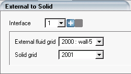
Click the button to save the configuration and close the window.
To launch CHT3D, right-click the main config icon of CHT3D_deicer, then select the option in the menu to launch the CHT3D calculation. In the execution environment, set the number of CPUs to
4for ICE3D and C3D.Note: The simulation progress can be monitored in the Log and Graphs panels.
To appropriately compare the results of this CHT de-icing simulation using Fluent with the kw-sst turbulence model, another CHT de-icing simulation using FENSAP with its own kw-sst turbulence model was conducted. Unsteady Electro-Thermal De-icing in Wet Air uses the Spalart-Allmaras turbulence model and therefore its results are not suitable to make proper comparisons. Therefore, results and comparisons of both kw-sst cases are presented in this subsection and show that Fluent and FENSAP produce similar CHT results.
The following graph shows the history of the maximum temperature of the solid domain throughout the simulation.
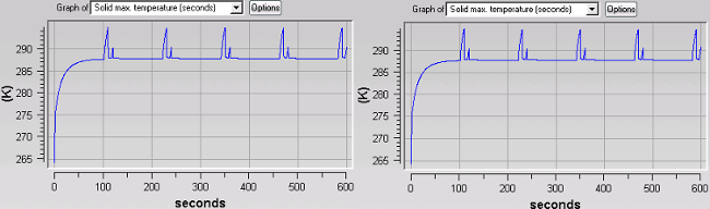
The following graph shows the history of the temperature at three locations on the surface compared to experimental data.
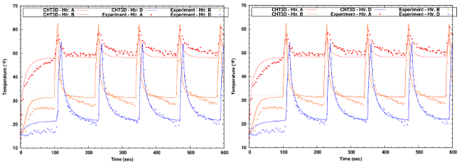
Figure 7.86: Residual Ice Shape and Solid Temperature at (a) 100, (b) 110, (c) 120 and (d) 220 Seconds; (Left: Fluent; Right: FENSAP)
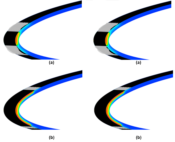
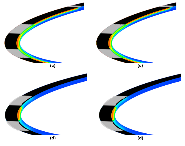
This tutorial demonstrates how to use C3D to compute the current and temperature rise in a heating element. A thermostat is used to regulate the maximum and minimum allowable temperature of the heating element.
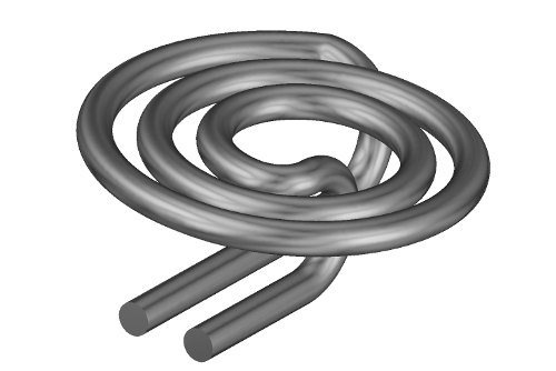
Open the FENSAP-ICE graphical interface and create a new project with the → menu or the New project icon. Name the project
c3d_electrothermal_heating. Select the metric unit system.Create a new C3D run with the → menu or the new run icon. Name this run
HEATING_ELEMENT.Right-click the grid icon and select the Define option. Navigate to the folder ../workshop_input_files/Input_Grid/C3D and select c3d_heating_element.grd. Press Open to load the new grid file.
Double-click the config icon to edit the input parameters.
Go to the Settings panel and set the initial Temperature to
293.15K. Enable the Electro-thermal model. Place a thermostat by double-clicking the Thermostats title bar and clicking the Add radio button. The X, Y and Z coordinates are-0.0075,-0.01and-0.004m respectively. The thermostat position in the computational grid can be seen by clicking on the cube icon located to the right of the Thermostats label.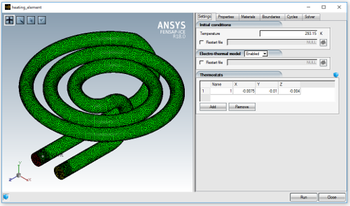
Go to the Properties panel. Rename the Default material to
Alloy. In this case, properties resembling nichrome will be used. Set the following properties for the alloy:Table 7.7: Electrical Conductivity
Distribution Temperature dependent Number of temperature points 3Temperature (K) Value (S/m) 293.151596588144110331035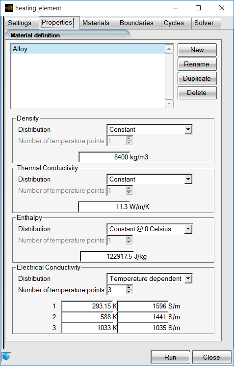
Go to the Materials panel. Select the material type for MAT_1 by choosing the Alloy in the Material type drop-down menu. Set the Thermostat to Enabled. Define the Minimum temperature and Maximum temperature as
810K and900K respectively. Skip the Boundaries panel. The boundary settings will be set when defining the heater cycle.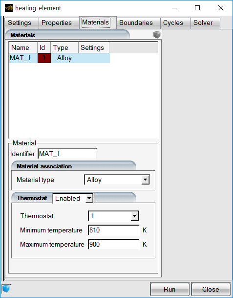
Proceed to the Cycles panel. Click
to add the first cycle, Cycle
A. Modify the Duration to 120s. Change BC in Current selection to Wall 2001. Set Thermal BC to Flux and Heat Flux to a constant value of0W/m2. Choose Voltage for Electrical BC and set a constant value of0V.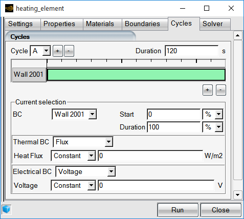
Add another BC within Cycle A by clicking
located under the cycle table. Select Wall 2002 in
the BC drop-down box of Current selection. Modify the
Voltage in Electrical BC to
240V.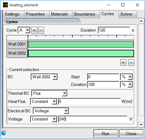
Finally, add the last boundary Wall 2003 by clicking
under the cycle table, set the Heat Flux to
-20000W/m2 to model the heat loss. Set Electrical BC to None.In the Sequence section, type cycle name A in the Cycles text box. Use
1Repetitions, and the Total time should be calculated automatically.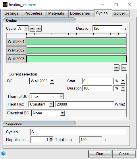
Go to the Solver panel. Set the Time step to Constant. Enter
0.5seconds in the Time step field and120seconds in Total time. Set the Iterations between printout to20. This prints the solution every 10 seconds.Click the button at the bottom of the window to go to the execution environment. Run this calculation on 4 processors. Set the number of CPU’s to
4if available and click Start to begin the calculation.Figure 7.87: Temperature at T=10s (20 Iterations), T=60s (120 Iterations) and T=110s (220 Iterations)
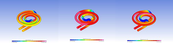
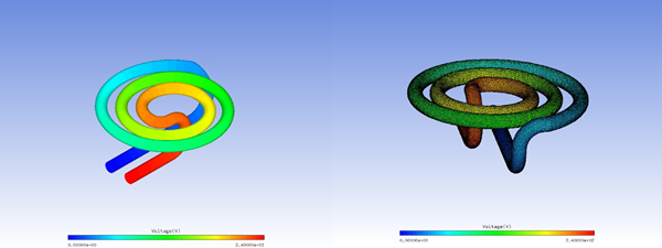
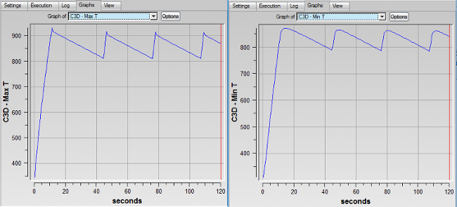
This tutorial illustrates the procedure to use CHT3D to compute the Conjugate Heat Transfer (CHT) through the metal skin of a nacelle lip, which separates the cold wet air flowing over the external skin surface from the hot internal air flow induced by the jet discharging from the orifice of the piccolo tube. To reduce computational effort, a rotational periodic axisymmetric nose cowl and a rotating engine nosecone are considered.
Typical flight conditions for an aircraft in holding configuration are chosen where the engine inlet cowl is subjected to an appendix D icing environment.
FENSAP-ICE’s approach to conjugate heat transfer consists of solving different domains separately, using a weak coupling technique. Therefore, FENSAP, DROP3D and ICE3D will be used to simulate the external cold wet air. C3D simulates the heat conduction through the nose cowl skin and FENSAP will be used to simulate the internal hot air flow.
Note: CHT3D can couple structured and unstructured grids without any limitations.
Once converged steady-state solutions are obtained on the fluid domains, heat transfer across fluid-solid interfaces are solved such that the temperature in the solid and fluid domains are updated after each CHT loop. This modularized approach provides some advantages:
It allows the work flow to be more streamlined and flexible. Different flow solvers (e.g. Fluent, CFX, etc.) can be used with CHT3D.
It allows for more robust convergence since one is given more freedom to define solver settings for each domain.
The smaller individual grid and solution file size for each domain makes post processing simpler.
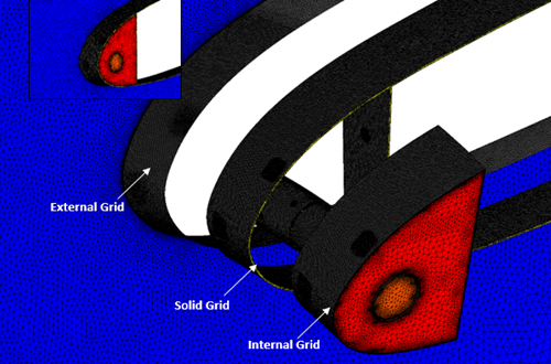
The tutorial proceeds in three steps:
Computing the external cold air flow with droplets and crystals.
Computing the internal hot air flow.
Conjugate heat transfer across the domains through the inlet cowl (nacelle lip, inner and outer barrel) skin.
Create a new project using → menu or the New project icon and name it
NACELLE_PICCOLO. Select the Metric units system.Create a FENSAP run in this project using the → menu or the New run icon and name it
FENSAP_ext.Double-click the grid icon and select the grid file nacelle_ext.grid provided in the tutorials subdirectory ../workshop_input_files/Input_Grid/CHT_nacelle.
The mesh is an unstructured grid with 1,054,220 nodes. The grid file contains the grid coordinates, the element connectivity table and the table of boundary surfaces.
Double-click the config icon to proceed to the input parameters setup.
Go to the Model panel. Select the Navier-Stokes option for the Momentum equations and Full PDE for the Energy equation.
Select the Spalart-Allmaras option for the Turbulence model and set the Eddy/Laminar viscosity ratio to
1e-5.Note: For anti-icing simulations, since no ice (roughness) is expected, Free transition model should be selected for external air flow calculations to capture the laminar flow regions more accurately. Otherwise, fully turbulent flow calculations, may overpredict the heat transfer coefficients.
One can activate this inside the Model panel under the Transition box and selecting Free transition. However, for this tutorial, a fully turbulent external flow calculation is performed.
Next, go to the Conditions panel and set the Reference conditions as follows:
Characteristic length 0.635mAir velocity
155m/sAltitude
22000ftAir static temperature
252.15K (-21 °C)Under Initial solution, select the Velocity components option from the pull-down menu. Set the Velocity X component to
155m/s (same as the reference Air velocity). The other velocity components should be set to0m/s.Go to the Boundaries panel. Select the inlet boundary BC_1001 and choose the Subsonic option under Type. Click the button to set the Inlet conditions.
Select the wall boundary BC_2011. Set Surface type to No-slip and set the Temperature value by right-clicking in the temperature box and Copy from… → Adiabatic stagnation temperature + 10.
Note: A wall temperature must be specified on the inlet cowl (BC_2011) to compute an initial wall heat flux to start the CHT calculation. This temperature will subsequently be updated automatically during the CHT3D loop.
Repeat the same settings for the family BC_2012 and BC_2013. Since BC_2013 represents an engine nosecone spinner, enable Rotation and impose a rotational speed of
4000rpm.Select the outflow boundary BC_3000. Choose the type as Subsonic, and click the button to set the exit pressure value to Reference conditions.
Select the outflow boundary BC_3001. Choose Mass flow under Type, and specify a mass flow rate of
1.54kg/s.Go to the Solver panel. Select the Steady option in the Time integration pull-down menu. Set the value of the CFL number to
200and the Maximum number of time steps to350. Click the Use variable relaxation check box and set300in Time steps.Note: This CFL number chosen for this case works well with the provided grid which is rather simple. For more complex configurations and larger pressure ratios, lower CFL numbers may be necessary for convergence. There is usually an optimum CFL number for each grid and conditions, which takes the solution to convergence fastest. Low CFL values will take longer to converge, while very high values can result in some unwanted oscillations in the transient solution (beginning of the iteration process) that will take additional time to clear out.
Choose the Streamline upwind option in the Artificial viscosity tab. Set the Cross-wind dissipation coefficient to
1.e-7and move the slider to 100% Second order position.Go to the Out panel. Save the Solution every 50 iterations in Overwrite mode. Activate Write Y+ to solution and output lift and drag coefficients by selecting Drag direction based on inlet BC in Forces. Set the Drag BC to 1001, the Positive lift direction to +Y, the Reference area to
0.279521162m2, and the Moment reference point -X, -Y, -Z to0.5265,0,0m.The calculations may take some time depending on the number of available CPUs. The converged solution is provided in the tutorials subdirectory ../workshop_input_files/Input_Grid/CHT_nacelle/soln_ext if you do not wish to wait for the results before proceeding to the next section of this tutorial.
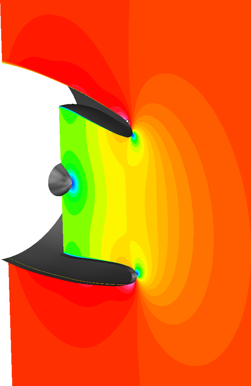
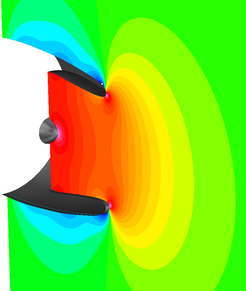
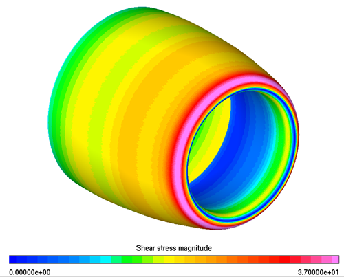
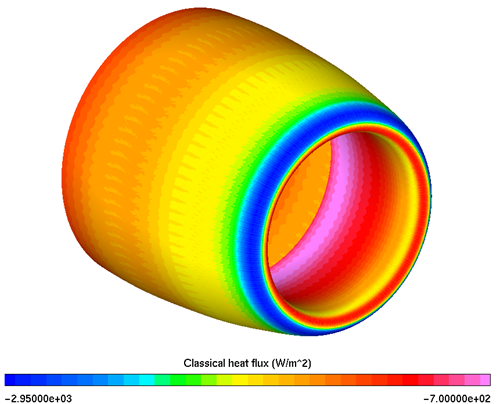
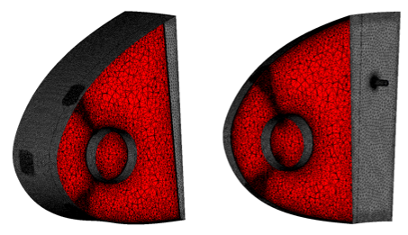
Create a new FENSAP run and name it
FENSAP_int.Double-click the grid icon to assign the grid file. Select the grid file nacelle_int.grid provided in the tutorials subdirectory ../workshop_input_files/Input_Grid/CHT_nacelle/. The mesh is an unstructured grid with 1,114,420 nodes.
Double-click the config icon to open the FENSAP input parameters window.
Go to the Model panel. Select the Navier-Stokes option for the Momentum equations (viscous flow) and Full PDE for the Energy equation.
Select K-omega SST as the Turbulence model and set the Eddy/Laminar viscosity ratio to
5and the Turbulence intensity to0.01.Go to the Conditions panel and set the following Reference conditions:
Characteristic length 0.005mAir velocity 84m/sAir static pressure 178452.02PaAir static temperature
511.47K (238.32°C)The Characteristic length setting has no impact on the flow, but it will change the scale of the average residual which is reported in non-dimensional form. A large characteristic length will make the average residual appear smaller. It is good practice to choose a characteristic length that matches the scale of the computational domain. In this case, 0.05m is the diameter of the piccolo tube.
Under Initial solution, select the Velocity components option from the pull-down menu. Set the three components of velocity to
0m/s.Next, each domain is initialized separately to improve convergence. Go to the Domains panel.
Select Domain_0. This domain represents the airflow inside the piccolo tube. Under Initialization, select Custom and set Velocity -X, -Y and -Z to
0,0,84m/s, Pressure to178,452.02Pa and Temperature to511.47K since this domain is strongly influenced by the conditions imposed at the inlet, BC_1000.Select Domain_1. This domain represents the airflow inside the D-duct. Under Initialization, select Custom and set Velocity -X, -Y and -Z to
0,0,0m/s, Pressure to42,830.57Pa and Temperature to400K. In general, initializing this cavity with 0 velocity and with the outlet static condition, BC_3000, is recommended as most of the airflow travels at a low speed inside the D-duct.
Go to the Boundaries panel. Select the inlet family BC_1000. Under Type, select the Engine inlet – Mass flow rate option from the pull-down menu and set the following conditions:
Total pressure 182800PaTotal temperature 515K (241.85 °C)Mass flow rate 0.200773kg/sAlpha 0degBeta 90degThe velocity vector is perpendicular to the inlet surface. This vector can be displayed in the Graphics window by clicking on
 at the right of the BC Inlet parameters tab.
Set the wall boundary conditions as follows:
BC_2000 No-slip Temperature 300K (26.85 ᵒC)BC_2001 No-slip Temperature 300K (26.85 ᵒC)BC_2002 No-slip Temperature 515K (241.85 ᵒC)BC_2003 No-slip Temperature 515K (241.85 ᵒC)BC_2004 No-slip Temperature 515K (241.85 ᵒC)BC_2005 No-slip Temperature 300K (26.85 ᵒC)Note: Temperature must be specified on the interfacing boundary condition families to initialize the CHT calculation between the two domains (internal hot air and skin). In this case, BC_2000 will interface with the nacelle lip skin, BC_2001 and BC_2005 will interface with the forward bulkhead, and BC_2002, BC_2003 and BC_2004 will interface with the piccolo tube skin. These temperatures will be updated automatically during the CHT3D loop, as conduction takes place through these skins.
Select the BC_3000 family and click the button under Type. Set the Pressure value to
42,830.57Pa. This is the exit pressure opening to the external free stream flow.Select the BC_3001 family and click the button under Type. Set the Pressure value to
178,452.02Pa. This is the exit pressure opening to the remaining portion of the piccolo tube.Go to the Solver panel. Select the Steady option in the Time integration pull-down menu. Set the value of the CFL number to
200and the Maximum number of time steps to600. Click the Use variable relaxation check box and set300in Time steps.Note: For this tutorial, the Maximum number of time steps were set to 600 to reduce the length of computational time. Together with the residual convergence plots, one should always check to see if the mass deficit convergence is less than 0.1% of the total incoming mass flow rate. In this case, the mass flow rate deficit was less than 0.5%. For increased accuracy, one can run the simulation for 2000 iterations.
Choose the Streamline upwind option under Artificial viscosity. Set the Cross-wind dissipation coefficient to
1.e-7and move the slider to 100% Second order position.Go to the Out panel. Save the Solution every 50 iterations in Overwrite mode and select Write Y+ to solution.
Click the button to switch to the execution window. Under the Settings tab, use
16or more CPUs if possible.This calculation may take a long time to complete depending on the number of CPUs available. The converged solution is provided in the tutorials subdirectory ../workshop_input_files/Input_Grid/CHT_nacelle/soln_int. If you do not want to wait for the run to finish, you can use this file to set-up your CHT3D calculation, see Conjugate Heat Transfer (Wet-Air Regime). The two main convergence indicators for this run are the average residual and the total heat flux. The run should be allowed to continue until the total heat flux converges well. The total heat flux curve should reach an asymptotic value of about 350 Watts. You can zoom on convergence curves by holding Shift and left-click. Middle-click to undo the zoom.
Figure 7.96: Mach Number Contours and Wall Shear Stress at θ=0.0435 Radian (Top), θ=0 Radian (Bottom)
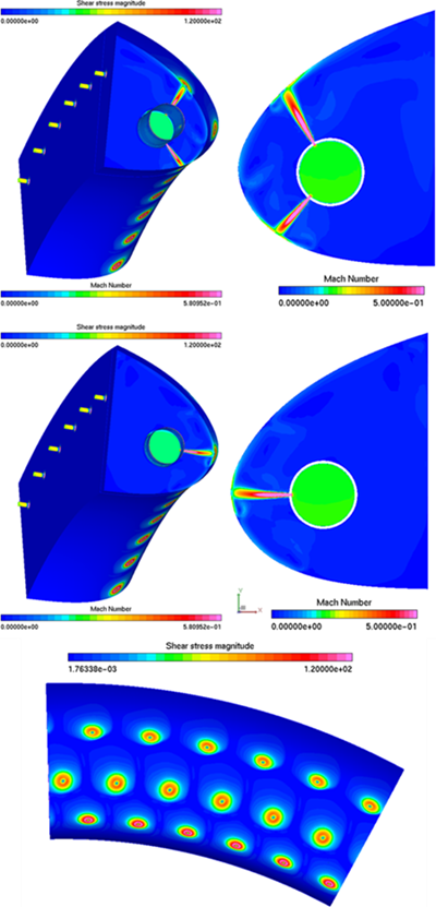
Figure 7.97: Jet Velocity Vectors Exiting from the Orifice, Showing the Complexity of the Internal Flow at θ=0 Radian (Left), θ=0.0435 Radian (Right)
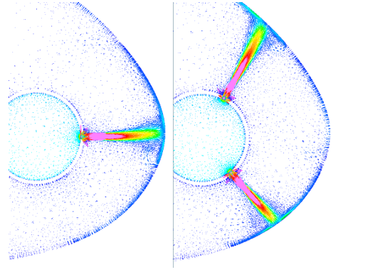
Figure 7.98: Total Temperature Contours and Wall Heat Fluxes at θ=0 Radian (Top), θ=0.0435 Radian (Bottom)
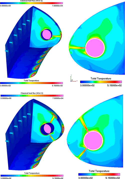
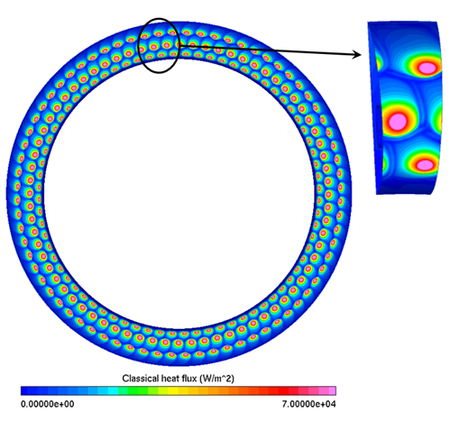
Create a new DROP3D run and name it
DROP3D_ext.Drag & drop the config icon of FENSAP_ext onto the config icon of the new DROP3D run. This copies the reference conditions of the flow to the droplet run.
Double-click the DROP3D_ext config icon to edit the parameters.
Go to the Model panel and under Particles parameters, set Droplets + Crystals as Particle type.
Next, go to the Conditions panel.
Set the following Droplet reference conditions:
Droplet diameter
20micronsWater density
1,000kg/m3Particles distribution Monodisperse
Set the following Ice crystals reference conditions:
Choose Appendix → Appendix D. Click Configure.
Liquid Water Content
0.5g/m3. The Ice Crystal Content automatically becomes3.52138167g/m3.
Crystal type → Solid thick plate. The Aspect ratio automatically becomes 0.3836.
Crystal density
917kg/m3Size
100microns
Under Particles initial solution, select Velocity components and set the Velocity -X, -Y, -Z to
155,0,0m/s.
Go to the Boundaries panel. Select the BC_1001 (Inlet) boundary condition and click the Import reference conditions button. Verify that the nosecone, BC_2013, is rotating at 4,000 rpm.
Go to the Solver panel. Set the CFL number to
20and the Maximum number of time steps to250. Decrease the Convergence level and Change in total beta to1e-12in the Advanced solver settings section.Note: For this tutorial, the Maximum number of time steps were set to 250 to reduce the length of computational time. Together with the residual convergence plots, one should always check to see if no change is observed in the Total Beta and Change in total Beta convergence for both droplets and crystals. For increased accuracy, one can run the simulation for 500 iterations. This may allow shadow and enrichment zones to develop further which can affect downstream components e.g. the spinner cone or other engine components.
Go to the Out panel. Save the Solution every
40iterations in Overwrite mode.Click the button. Start the calculation on
16or more CPUs if possible.The calculations may take some time depending on the number of available CPUs. The converged solutions are provided in the tutorials subdirectory ../workshop_input_files/Input_Grid/CHT_nacelle/droplet ../workshop_input_files/Input_Grid/CHT_nacelle/crystal if you do not wish to wait for the results before proceeding to the next tutorial.
Figure 7.101: Collection Efficiency of Droplets (Left) vs Crystals (Right) on the Engine Nacelle Lip & Nosecone
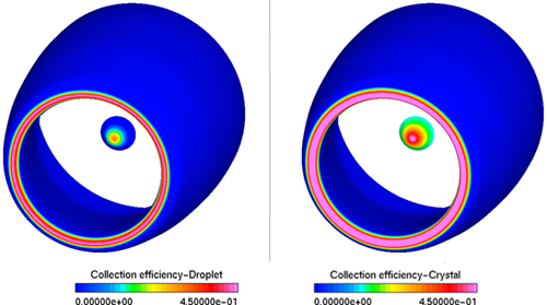
The ice crystals are larger than the water droplets and therefore exhibit a more ballistic nature (less entrained by the airflow). This difference is shown in Figure 7.100: Droplet LWC (Left) and Crystal ICC (Right) on the External Flow as ice crystals tend to produce larger shadow and enrichment zones than water droplets as well as in Figure 7.101: Collection Efficiency of Droplets (Left) vs Crystals (Right) on the Engine Nacelle Lip & Nosecone as ice crystals generate wider impingement regions and have higher collection efficiencies than water droplets.
Note: Due to the stream tube effect, the engine nacelle lip and the engine nosecone have a considerable impact on the total water content and its distribution that goes into the engine.
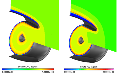
The goal of this step is not to provide an initial ice shape, but rather to establish a water film on the outer surface of the solid as an initial condition for the wet CHT3D run.
Create a new ICE3D run and name it
ICE3D_ext.Drag & drop the config icon of the DROP3D_ext onto the config icon of this new run. This operation automatically links the air, droplet and ice crystal solutions, as well as the grid of the external domain and the reference conditions to the ICE3D_ext run.
Double-click the config icon to edit the input parameters.
Go to the Model panel. Under the Icing model, select Glaze – Advanced for Ice-Water Model and change the Heat flux type to Classical.
Under Ice crystals, choose Droplets+Crystals from the pull-down menu to activate both droplets and ice crystals. Under Modes select NTI bouncing model as the particle bouncing model. This model adds the effect of ice crystals surface collision dynamics to the ice shape.
Go to the Conditions panel and set the Recovery factor to 0.9. The remaining settings were automatically transferred from the DROP3D_ext configuration.
Go to the Solver panel. Keep the Automatic time step option enabled and change the Total time of ice accretion to
30seconds.Run the calculation on
8or more CPUs if possible.For comparison, a separate ICE3D simulation without ice crystals was simulated using the same in-flight icing condition of this tutorial by disabling the ice crystals in the Model panel. The following figures show the mass caught, water film distributions and ice accretion rate of these two simulations.
Figure 7.102: Mass Caught Droplets Only (Left) vs Droplets+Crystals (Right) on the Engine Inlet Cowl & Nosecone and Figure 7.104: Instant Ice Growth Droplets Only (Left) vs Droplets+Crystals (Right) on the Engine Inlet Cowl & Nosecone reveal that in presence of water film on the surfaces of the nacelle cowl and nosecone, ice crystals would stick resulting in an increase of the total mass of water caught and total ice accretion rate. In return, this extra mass of ice increases local cooling effects thus reducing the amount and extent of water film over the nacelle lip (Figure 7.103: Film Thickness Droplets Only (Left) vs Droplets+Crystals (Right) on the Engine Inlet Cowl & Nosecone).
Note: If the engine nacelle was exposed to a cloud of crystals only, no water catch would be observed on the surface since all ice crystals would bounce off the dry surface. For crystals to stick on the surface, water film must be present on the surface or, prior to impact, melting of crystals would need to take place.
Figure 7.102: Mass Caught Droplets Only (Left) vs Droplets+Crystals (Right) on the Engine Inlet Cowl & Nosecone
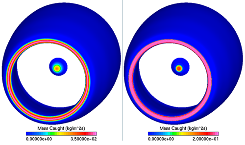
Figure 7.103: Film Thickness Droplets Only (Left) vs Droplets+Crystals (Right) on the Engine Inlet Cowl & Nosecone
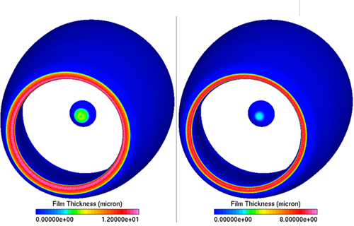
Figure 7.104: Instant Ice Growth Droplets Only (Left) vs Droplets+Crystals (Right) on the Engine Inlet Cowl & Nosecone
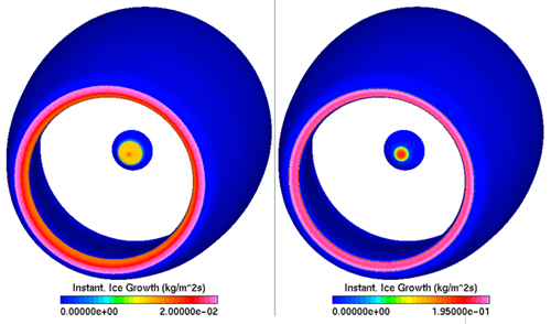
This section illustrates the Conjugate Heat Transfer procedure (CHT3D) that is used to couple the external, solid and internal domains to determine the equilibrium temperature distribution in all domains. In this case, the energy equation of water droplets and crystals are enabled to predict potential phase change of ice crystals and evaporation of water droplets.
Create a new CHT3D run and name it
CHT3D_wet. The CHT configuration prompt window will open showing different CHT simulation types. Select Piccolo (2 fluids, 1 solid) in the Problem type pull-down menu, then choose Wet air & droplets. Press the button to continue with the set-up. A tree of coupled FENSAP, DROP3D, ICE3D and C3D runs will appear in the run window.Note: For this tutorial, a simple Wet air simulation could have been selected as the heated nacelle lip barely changes the state of droplets and crystals. These changes are observed mainly in the thermal boundary layer. By choosing Wet air, the simulation time decreases as DROP3D is not part of the CHT simulation. Usually, Wet air & droplets simulations are for problems that experience large changes in temperature such as engine compressor components and heated pitot tubes. In the case of pitot tubes, chances for water droplets to evaporate and crystals to melt are high as particles get closer to the tube and therefore phase change will influence the total amount of water collected by the tube.
Drag & drop the config icon of FENSAP_ext onto the config icon of the fluid_ext run in CHT3D_wet.
Double-click the config icon of the fluid_ext run to edit the input parameters.
Go to the Solver panel. Change the CFL number to
1,000and the Maximum number of time steps to50. Uncheck Use variable relaxation. In the Advanced solver settings section, decrease the Convergence level of Convergence criteria to1e-20.Close and save the configuration file.
Drag & drop the config icon of DROP3D_ext onto the config icon of the drop_ext run in CHT3D_wet.
Double-click the config icon of the to the drop_ext run to edit the input parameters.
Go to the Model panel. In Particles parameters, enable Particle thermal equation. Activating this option will allow the computation of a temperature field for water droplets and ice crystals. This will also account for ice crystals phase change by computing the melting fraction which in turn will change the overall particle behavior before and on impact on the surfaces.
Go to the Solver panel. Keep the CFL number to
20and change the Maximum number of time steps to50. Close and save the configuration file.Drag & drop the config icon from ICE3D_ext onto the config icon of the ice_ext run in CHT3D_wet. No modifications to the configuration of this run are required.
Drag & drop the config icon of FENSAP_int onto the config icon of the fluid_int run in CHT3D_wet.
Double-click the config icon of the fluid_int run to edit the input parameters.
Go to the Solver panel. Change the CFL number value to
1,000and the Maximum number of time steps to50. Disable the Use variable relaxation check box. In the Advanced solver settings section, decrease the Convergence level of Convergence criteria to1e-20.Close and save the configuration file.
To configure the solid run in CHT3D_wet, double-click the grid icon and select the file nacelle_skin.grid provided in the tutorials subdirectory ../workshop_input_files/Input_Grid/CHT_nacelle.
Double-click the config icon of the solid run to edit the input parameters for skin heat conduction.
Go to the Settings panel. Set the Temperature to
264.1K. This will be the initial temperature throughout the solid domain.Go to the Properties panel. Click the Rename button to rename Default material to
Aluminum
       2090-T86
and create the following materials and their corresponding properties.Material Definition:
Aluminum 2090-T86Density (Distribution: Constant) 4,430kg/m3Thermal Conductivity (Distribution: Constant) 6.7W/m/KEnthalpy (Distribution: Constant @ 0 Celsius) 143,758.85J/kgAluminum 2219-T81Density Distribution: Temperature dependent
Number of temperature points: 4
273.15K2,703kg/m3371.15K2,685kg/m3474.15K2,657kg/m3589.15K2,630kg/m3Thermal Conductivity Distribution: Temperature dependent
Number of temperature points: 4
273.15K162W/m/K371.15K177W/m/K474.15K192W/m/K589.15K207W/m/KEnthalpy Distribution: Temperature dependent
Number of temperature points: 4
273.15K250,478.55J/kg371.15K343,333.55J/kg474.15K446,642.55J/kg589.15K567,737.55J/kgCompositeDensity (Distribution: Constant 2,070kg/m3Thermal Conductivity (Distribution: Constant) 0.84W/m/KEnthalpy (Distribution: Constant @ 0 Celsius) 218,520J/kgTitanium 6Al-4VDensity (Distribution: Constant 4,430kg/m3Thermal Conductivity (Distribution: Constant) 6.7W/m/KEnthalpy (Distribution: Constant @ 0 Celsius) 143,758.85J/kgTitanium Ti-6Al-6V-2SnDensity (Distribution: Constant 4,540kg/m3Thermal Conductivity (Distribution: Constant) 6.6W/m/KEnthalpy (Distribution: Constant @ 0 Celsius) 183,010.5J/kg
Go to the Materials panel. Select the Material type for each region of the grid.
MAT_1 = Aluminum 2219-T81
MAT_2 = Composite
MAT_3 = Aluminum 2090-T86
MAT_4 = Titanium 6Al-4V
MAT_5 = Titanium Ti-6Al-6V-2Sn
Go to the Boundaries panel. Define the boundary conditions of the surfaces of the solid as follows:
BC_2000 to BC_2005: Default settings (Thermal BC definition set to Nothing)
BC_2010 and BC_2020 to BC_2051: Set Thermal BC definition to Type: Flux, and set Heat flux to
0W/m2.BC_2011: Default settings (Thermal BC definition set to Nothing).
BC_2000 to BC_2005 and BC_2011 are interface walls that will exchange information with the internal grid and the external grid respectively. CHT3D will automatically update theses boundary conditions during the simulation.
Go to the Solver panel. Set the Time step to Automatic. Set the Maximum time step value to
0.1seconds and the Total time to5seconds. At each CHT3D iteration, heat conduction will be computed for 5 seconds. Close and save this configuration.C3D total time per CHT3D iteration can be considered as the overall time step of the conjugate heat transfer problem. Reducing this value will improve the stability of CHT runs while increasing it may hinder convergence to a steady state temperature distribution in the solid.
Note: You may decide to set the Time step to Constant instead of Automatic. Depending on the simulation, this may or may not speed up the simulation, but may also reduce the stability of the simulation.
Double-click the main config icon of CHT3D_wet to set up the links between the solid and fluid domains.
Go to the Parameters panel. Set the Number of CHT iterations to
50and Solution output every0iterations (default value).Choose the Solve energy only option in the Flow solver mode pull-down menu for both internal and external flows.
The number of CHT iterations was set to 50 loops. It may be that you need more iterations to ensure full convergence of solid and ice solutions. In particular, the solid back plate temperatures may take longer to converge. Together with the convergence plots, it’s always advisable to check the evolution of the solution to see if any visible changes in temperatures can be seen.
Go to the Interfaces panel. There are seven fluid/solid interfaces in the computational domain. CHT3D will automatically exchange the boundary conditions between these three interfaces. Set up the interfaces as follows:
For External to Solid: There is only one interface between the external domain and the solid. Set the interface boundaries as follows:
Interface: 1
External fluid grid: 2011
Solid grid: 2011
Note: To easily identify which boundary condition interface with one another, click
 to highlight the boundaries for both solid and fluid domains that you
have selected in the graphical display window.
to highlight the boundaries for both solid and fluid domains that you
have selected in the graphical display window.For Solid to Internal: There are six interfaces between the solid and the internal domain. Set the interfaces as follows:
Interface: 1
Solid grid: 2000
Internal fluid grid: 2000
Then click the
button next to the Interface label to add extra
Solid to Internal interfaces:Interface: 2
Solid grid: 2001
Internal fluid grid: 2001
Interface: 3
Solid grid: 2002
Internal fluid grid: 2002
Interface: 4
Solid grid: 2003
Internal fluid grid: 2003
Interface: 5
Solid grid: 2004
Internal fluid grid: 2004
Interface: 6
Solid grid: 2005
Internal fluid grid: 2005
Note: In this case, the interface boundary condition family numbers across the two grids are adjusted so that they match, which is not a requirement. The only requirement is that the interface boundary conditions overlap nicely, with no gaps and discontinuities. They do not have to be node-to-node matching either.
Go to the Temperatures panel. The value of Recovery factor cannot be modified, the recovery factor of ICE3D will be used instead. Close and save the configuration.
Right-click the main config icon of CHT3D_wet, then select the option in the menu to launch the CHT3D calculation. Use
16or more CPUs for all solvers if possible and launch the calculation.Figure 7.105: Convergence History of the Maximum (Left) and Minimum (Right) Solid Domain Temperatures
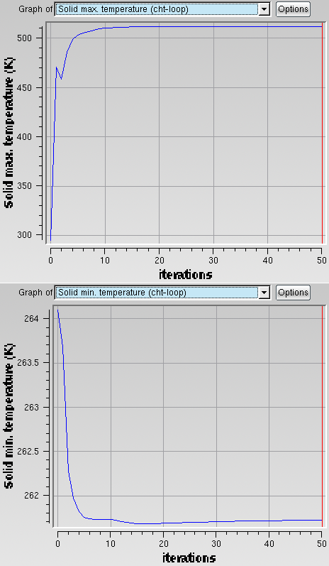
For comparison, a separate CHT3D simulation without ice crystals was simulated using the same in-flight icing and bleed air conditions used in this tutorial. The following figures show the temperature, water film thickness and ice accretion rate contours of these two CHT simulations.
Figure 7.106: Temperature Contours on the Solid (C3D) and Water Film Thickness and Ice Accretion Rate on the External Surface (ICE3D) – Droplets Only (Left) and Droplets + Crystals (Right)
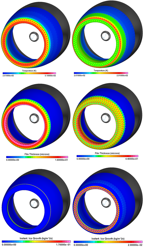
Figure 7.106: Temperature Contours on the Solid (C3D) and Water Film Thickness and Ice Accretion Rate on the External Surface (ICE3D) – Droplets Only (Left) and Droplets + Crystals (Right) shows that the combined droplets + ice crystals has a major impact on the heated nacelle lip icing. This is primarily due to the very high TWC of the droplet + crystal (4 g/m3) case compared to the droplet only (0.5 g/m3 ) case, leading to 8x more particle catch while the IPS is off (See Figure 7.102: Mass Caught Droplets Only (Left) vs Droplets+Crystals (Right) on the Engine Inlet Cowl & Nosecone). When heat is applied, water runback extends the wetted area where additional crystals stick, leading to residual icing on a larger portion of the engine inlet. The differences in temperatures are further apparent in Figure 7.107: Temperature Distribution vs. Wrap Distance on the Engine Inlet Cowl for Wet Air (Droplets + Crystals) and Wet Air (Droplets Only) Runs at θ=0 Radian (Left), θ=0.0435 Radian (Right). The extra ice coverage past the original impingement limits of droplets extends beyond the protected zone. This can be seen more clearly in Figure 7.108: 60 Seconds Runback Ice on the External Surface (ICE3D) – Droplets + Crystals. Such runback ice is a potential risk for engine core or airframe damage if ice shedding occurs. To simulate the runback ice shapes, drag & drop the config icon of the ice_ext run of the CHT3D_wet onto the config icon of a new ICE3D_post_CHT run. Change the Total time of ice accretion to
60seconds for example and run the calculation.Figure 7.107: Temperature Distribution vs. Wrap Distance on the Engine Inlet Cowl for Wet Air (Droplets + Crystals) and Wet Air (Droplets Only) Runs at θ=0 Radian (Left), θ=0.0435 Radian (Right)
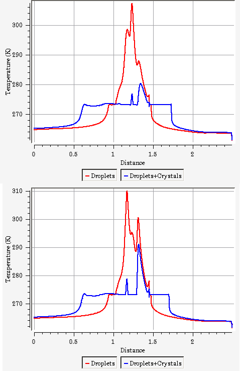
Another point to take note off is the melting of ice crystals in the vicinity of the engine nacelle lip. By changing its state, these liquid ice crystals no longer require a film of water to stick to the surfaces of aft aircraft components and will behave more like water droplets, contributing directly to ice formation. See Figure 7.109: Ice Crystals Melting - Liquid Phase of Ice Crystals on the External Domain (DROP3D).
Figure 7.110: FENSAP-ICE Demonstration of Multiphysics Holding Flight Calculations of an Engine Nacelle Anti-Icing System in an Appendix D Environment