


The following sections of this chapter are:
- 2.1. Computing Aerodynamic Coefficients on an ONERA M6 Wing at a Range of Angles of Attack
- 2.2. Computing Aerodynamic Coefficients and Wall Heat Flux on a Re- Entry Capsule at Different Altitudes in Earth and Mars Atmospheres Using Mixtures
- 2.3. Introduction to Aircraft Component Groups and Computing Aerodynamic Coefficients on an Aircraft at Different Flight Altitudes and Engine Regimes
- 2.4. Computing Aerodynamic Coefficients on an Aircraft Horizontal Tail Wing in a Wind Tunnel Domain at Different Mass Flow Rates
- 2.5. Fluent Aero AET – Creating a VBM Input File for Blade Sections
The objective of this tutorial is to use Fluent Aero to obtain lift, drag and moment coefficients on an ONERA M6 swept wing geometry at a range of angles of attack. This part of the tutorial will focus on using the Fluent Aero GUI to complete the setup, calculation and post processing of the multiple design points in the simulation.
Download the fluent_aero_tutorial.zip file here .
Unzip fluent_aero_tutorial.zip to your working directory.
Extract the oneram6-wing.msh.h5 file and the reference_data folder for this tutorial. The reference_data folder contains several .csv formatted text files. Their content will be compared to the CFD results of the current calculation. The reference data files are provided for demonstration purposes only.
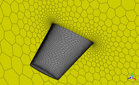
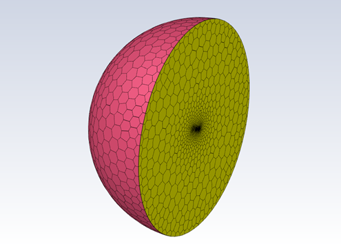
The oneram6-wing.msh.h5 file contains a grid of an ONERA-M6 swept wing that is an all-poly mesh and consists of 478,848 nodes, and 114,219 cells. This is a very coarse grid. Its purpose is to ease calculation time and resources while demonstrating the most common features of Fluent Aero. Four layers of prisms are grown off the wing’s wall boundaries and are used to capture the boundary layer. This number is insufficient if the goal is to obtain precise and accurate solutions. The limits of the computational domain are defined by a hemispherical boundary that acts as a pressure-farfield, and a flat circular boundary defined as a symmetry plane in the Z direction. This mesh follows the Freestream domain type requirements of a Fluent Aero simulation. For a Freestream domain type, the external boundary of the domain should be defined with a pressure-far-field zone, and can optionally include a connected pressure-outlet zone. Refer Freestream or WindTunnel Domain Type Requirements for more information.
Launch Fluent 2024 R2 on your computer. On the Fluent Launcher panel, set the Capacity Level to . Then select Aero. Set the number of Solver Processes to
4-8. Click .Alternatively, Fluent Aero can be opened using the aero (on Linux) or aero.bat (on Windows) file inside the fluent/bin/ folder.
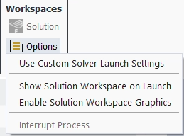
In the Fluent Aero workspace, go to the Project ribbon. Click Workspaces → , and make sure to uncheck , , and .
In the Project ribbon panel, select Project → and enter
Fluent_Aero_Tutorial_01to create a new project folder.In the Project ribbon, select Simulation → , and browse to and select the oneram6-wing.msh.h5 file. A New Simulation window will appear. Enter the Name of the New Simulation as
oneram6-aoa-exploration, and check . Click .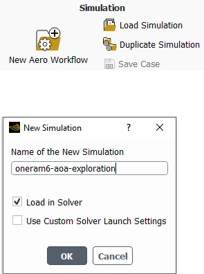
The case file will open and a background solver session will load. A new simulation folder will be created in your project folder. Fluent Aero will convert the .msh.h5 grid file to a .cas.h5 format case file and the latter will be imported in the simulation folder as oneram6-wing.cas.h5.
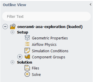
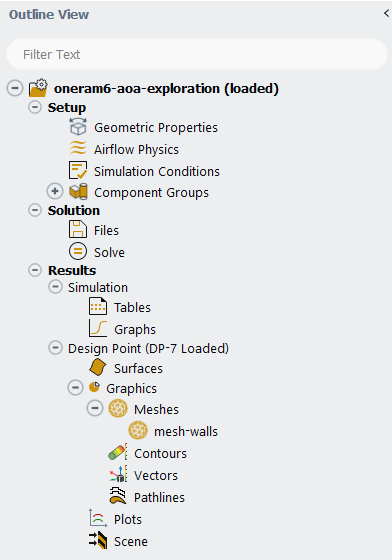
After the .cas.h5 file has been successfully loaded, a new Outline View tree appears under oneram6_aoa_exploration (loaded).
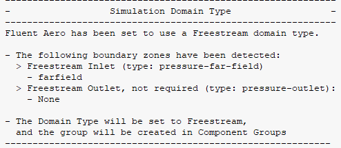
While importing, Fluent Aero will search for and find the pressure-far-field zone that defines the external boundary of the domain. If present, this will cause Fluent Aero to determine that this case is using a domain type, and the following message will be reported in the Console.
In the Outline View window, click Geometric Properties. A Properties - Geometric Properties window appears below the Outline View window. At the top of this new properties window, notice that the Domain Type has been automatically set to .
Define the orientation of the geometry within the computational domain, which will be used to compute the aerodynamic forces.
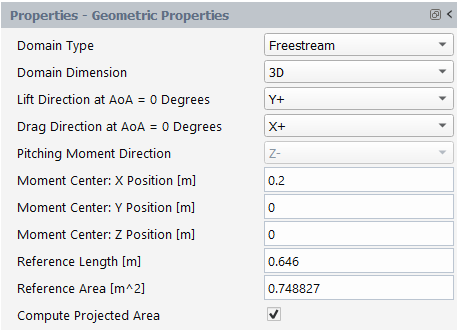
Set Domain Dimension to .
Set Lift Direction at AoA = 0 Degrees to .
Set Drag Direction at AoA = 0 Degrees to .
Set the Moment Center X, Y and Z Position [m] to
0.2,0, and0, respectively.Set the Reference Length [m] to
0.646, which corresponds to the mean chord length.Set the Reference Area [m^2] to
0.748827.
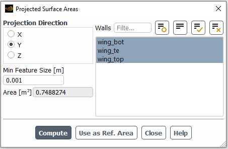
Alternatively, the reference area can be computed by enabling the option. A Projected Surface Areas dialog will appear. Set the Projection Direction to and select all wall surfaces. Click the button and then click the button to copy the computed area to the Reference Area [m^2] box.
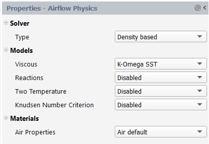
In the Setup tree, go to Airflow Physics. A Properties – Airflow Physics window appears below the Outline View window.
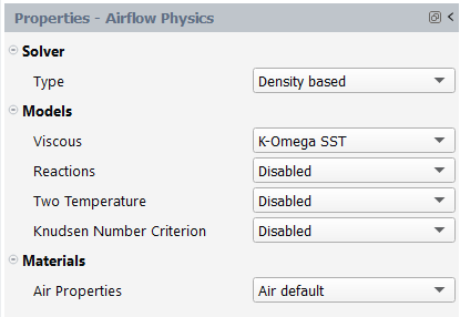
In the Solver section:
Set Type to .
In the Models section:
Set Viscous to .
Set Reactions to .
Set Two Temperature to .
Set Knudsen Number Criterion to .
In the Materials section:
Set Air Properties to .
In the Setup tree, go to Simulation Conditions. In the Properties – Simulation Conditions window, go to Flight Conditions.
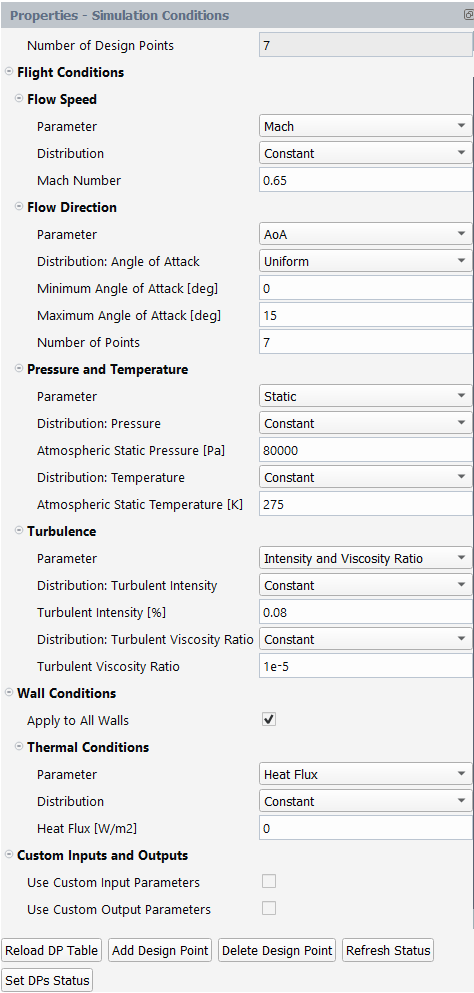
In the Flow Speed section,
Set Parameter to .
Set Distribution to .
Set the Mach Number to
0.65.
In the Flow Direction section,
Set Parameter to .
Set Distribution: Angle of Attack to .
Set the Minimum Angle of Attack [deg] to
0.Set the Maximum Angle of Attack [deg] to
15.Set the Number of Points to
7.
In the Pressure and Temperature section,
Set Parameter to .
Set Distribution: Pressure to .
Set the Atmospheric Static Pressure [Pa] to
80000.Set Distribution: Temperature to .
Set the Atmospheric Static Temperature [K] to
275.
In the Turbulence section:
Set Parameter to .
Set both Distribution: Turbulent Intensity and Distribution: Turbulent Viscosity Ratio to .
Set Turbulent Intensity [%] to
0.08.Set Turbulent Viscosity Ratio to
1e-5.
In the Wall Conditions section:
Enable .
In the Thermal Conditions section:
Set Parameter to .
Set Distribution to .
Set Heat Flux [W/m2] to
0.
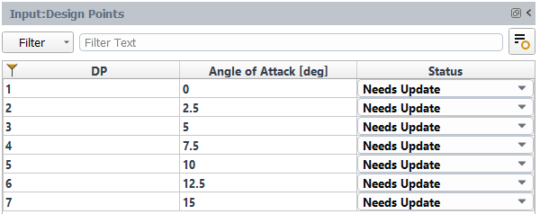
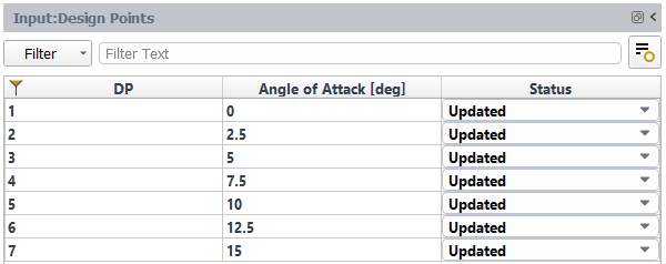
An Input:Design Points table will be created in the Graphics window on the right-hand side of the user interface. This table shows all the design points that will be simulated. The initial status of each design points (DP) has been set as . The status can be set as if you decide not to update one or several design points. In this tutorial, you will keep all design points as .
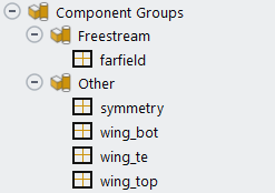
Go to Component Groups. Two default Component Groups have been created after the simulation is loaded.
The group contains the pressure-far-field zone that defines the external boundary of the domain and is where the freestream atmospheric flight conditions for each design point are defined as boundary conditions.
The Other group contains the remainder of the boundary zones which are the walls of the oneram6 wing geometry and the symmetry plane of the simulation domain.
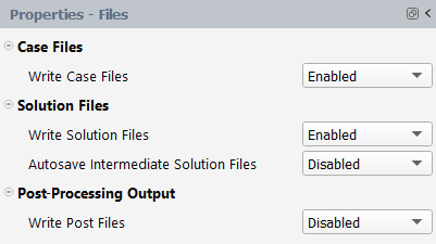
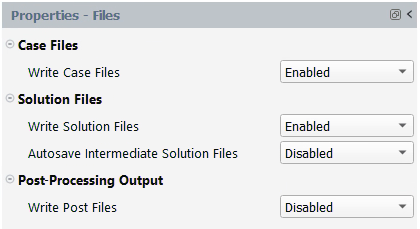
In the Outline View, go to Solution → Files. This step allows you to control the output files written per design point. Keep the default options.
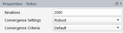
Under Solve, keep the default number of Iterations of
1000. Keep both Convergence Settings and Convergence Criteria as .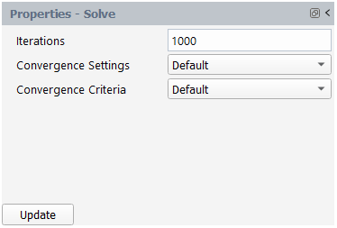
Click the button at the bottom of the Properties - Solve panel.
The calculation will start, and the first design point, DP-1, featuring the minimum Angle of Attack, will be simulated. A Convergence window will appear in place of the Graphics window and display the residuals and monitors for DP-1.
Design point DP-1 will calculate until the total Iterations (1000) or the Residuals Convergence Cutoff (1e-5) and Aero Coeff Conv. Cutoff (2e-5) are reached, whichever comes first. In this example, DP-1 will calculate for about
350iterations. At that point, the Angle of Attack will be updated for the next design point and the calculation will resume. This process repeats until all design points are simulated.Moreover, in the Project View, a Results folder will be created after the calculation starts. A folder for each design point along with an associated case file, data file, and convergence file will appear inside the Results folder.
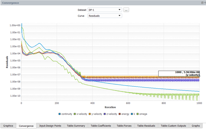
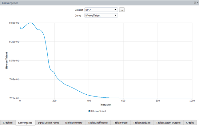
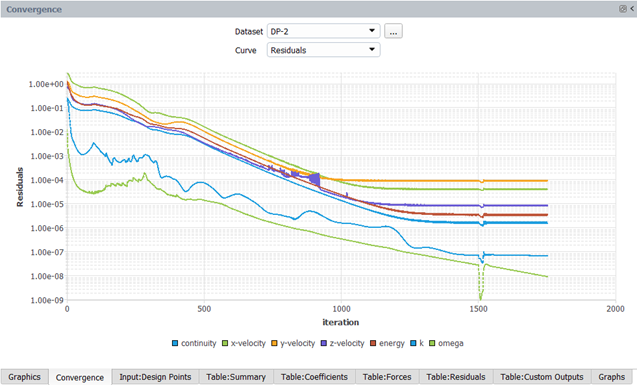
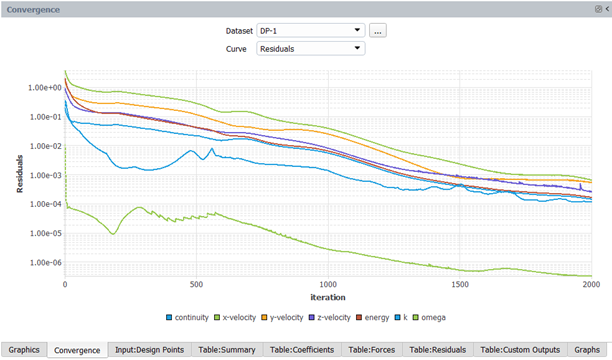
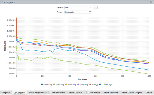
Examine the simulation's convergence history in the Convergence window, which is located on the right side of your screen. Set the Dataset to and the Curve to , to view the continuity, x-, y-, z-velocity, energy, and turbulence residuals for the first design point. You can left-click a residual curve to show the iteration number and the corresponding residual value. Here, the residual y-velocity at iteration 1000 is shown and equals to 5.90306e-8. The calculation has ended after reaching the maximum number of iterations.
Note: While all residuals in the image above meet the residual convergence cutoff criterion of 1e-5, it is still recommended for you to investigate your solutions to ensure that appropriate convergence levels have been achieved and that convergence remains stable. A residual convergence cutoff of 1e-5 may be appropriate for some cases, but not for others, and therefore care should be taken when selecting this value. If a stricter convergence criterion is required, you can go to Solve, change Convergence Criteria to and set a lower value (
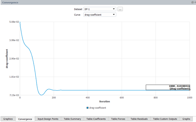
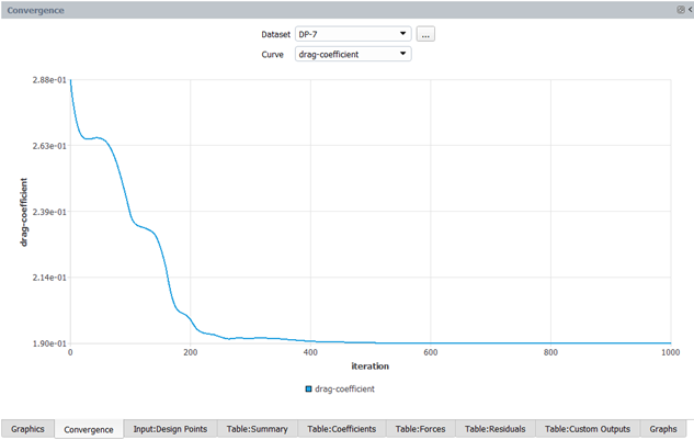
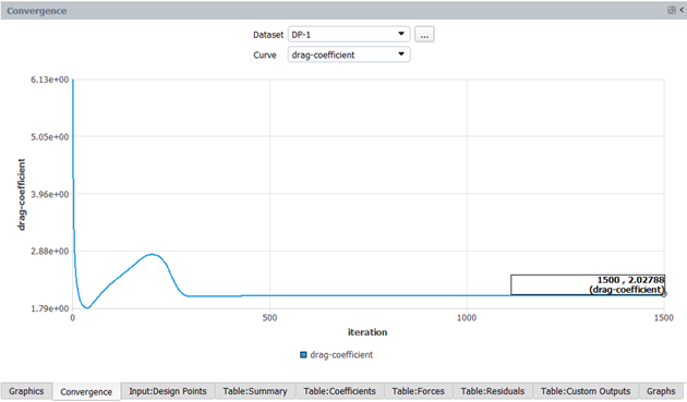
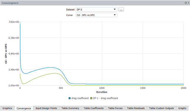
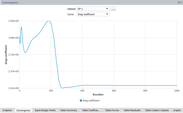
1e-6for example) next to Residuals Convergence Cutoff.In the Convergence window, set Curve to . The evolution of the drag coefficient for DP-1 will be displayed. Left-click the last iteration of the drag-coefficient plot, to show the drag coefficient value.
When the calculation of DP-1 is complete, the status column in row 1 of the Input:Design Points table will be set to , and the calculation of DP-2 will begin.
After all the design points have been updated, the status of the Input:Design Points table will be set to for all the design points.
A Results node will be displayed in the Outline View tree after the simulation starts. The Results node contains a Simulation and a Design Point sub-components.This allows you to quickly post-process design point solutions, by obtaining aerodynamic coefficient plots, creating contour plots of solution fields, comparing solution fields to experimental data, and more.
Go to the Simulation node. This node provides a comprehensive view of aerodynamic coefficients across all design points. The first element in the Simulation node is Tables. In the current tutorial, 4 different Tables will be created automatically in the Graphics window area when the calculation is complete.
Click the Table:Summary, Table:Coefficients, Table:Forces and Table:Residuals tabs at the bottom of the Graphics window to reveal each table.
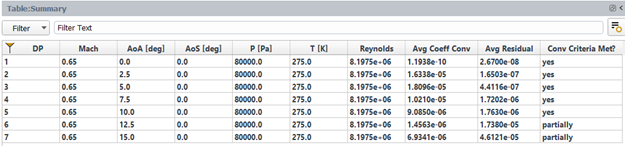
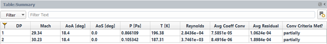
Table:Summary summarizes the flight conditions and convergence information for each design point. In the current simulation, most design points have met or partially met the convergence criteria.
Note: Depending on the number of CPUs used to calculate the design points, there may be some differences in the convergence achieved.
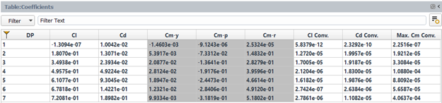
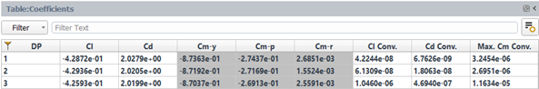
Table:Coefficients contains lift and drag coefficients calculated in wind-fixed coordinate systems, as well as yaw, pitching, and rolling moment coefficients calculated in body-fixed coordinate systems, which are highlighted in gray. Display Aero Forces in the Properties - Tables panel can also be changed to show forces and moments in the body-fixed, wind-fixed, or both coordinate systems at the same time. The convergence of the lift and drag coefficients is measured by the Cl Conv. and Cd Conv. columns. These are used to determine whether or not the convergence criteria have been met. The maximum value of the convergence of the yaw, pitching, and rolling moments is shown in the last column, Max. Cm Conv..
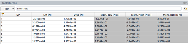
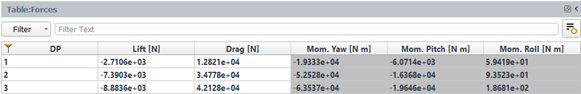
Table:Forces contains the lift, drag and moment forces. Coefficients, lift, and drag forces are computed in the wind-fixed coordinate system, while moment forces are computed in the body-fixed coordinate system.
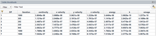
Table:Residuals shows the final residuals as well as the number of iterations run for each design point.
Based on the convergence status, you can continue to calculate selected design points from the current results. Although the convergence criteria have been partially met for design points 6 and 7, which have high angle of attacks, the average residual and the residual of aerodynamic coefficients are very low. The aerodynamic forces plateaued after 600 iterations, as shown in Figure 2.11: Convergence History of the Lift Coefficient for Design Point 7 and Figure 2.12: Convergence History of the Drag Coefficient for Design Point 7.
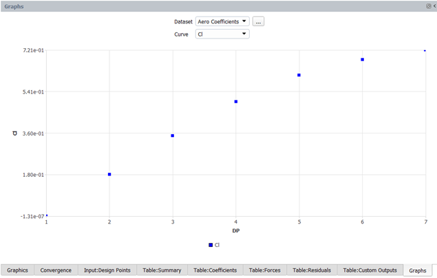
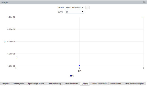
Click Graphs in the Outline View to show the plots of the aerodynamic coefficients defined in Fluent Aero. At the bottom of the Properties - Graphs window, click Plot Coefficients.
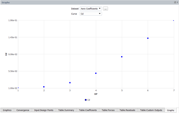
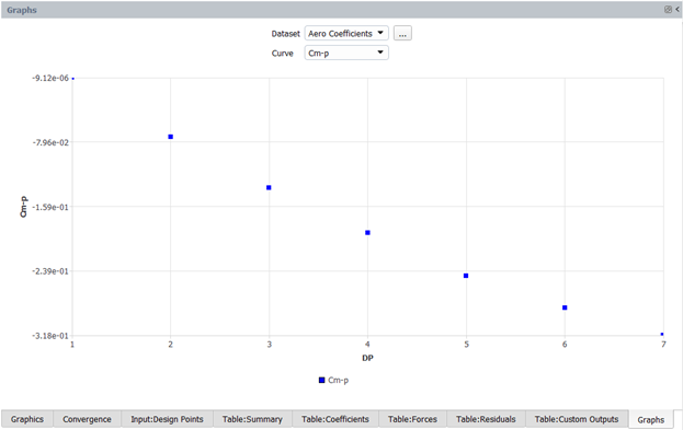
An X- Y plot of lift coefficient () vs. design point () will appear in the Graphics window. The drag and moment coefficients can be shown by selecting and from the Curve selection drop-down list.
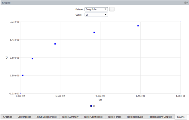
Click the button. An X-Y plot of Lift Coefficient (Cl) vs. Drag Coefficient (Cd) will appear in the Graphics window. Alternatively, you can simply change Dataset to from the Graphics window to show the drag polar plot.
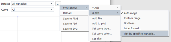
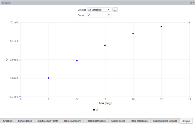
Click the button. An X-Y plot AoA vs. DP will appear in the Graphics window. Select from the Curve drop-down. There is an option button located on the right of the Dataset drop-down. This button can be used to modify some of the plot settings and export the plot to the disk. Click the option button and select → → to change the x variable to AoA. The plot of the lift coefficient vs the angle of attack will be shown.
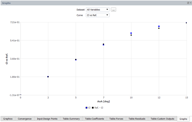
In the Properties – Graphs window, you can load and plot a reference dataset to compare with the simulation results by using the function. To compare the Cl vs AoA curve from simulation with a reference data, set Dataset to and Curve to from the Graphs plot window. Ensure that AoA is the x-axis variable. Click . A file browser will appear. For this tutorial, you will use the results from a finer mesh to demonstrate this functionality. Browse to the reference_data folder inside the tutorial folder and select the ref-onera-wing-Cl-vs-AoA.csv file. The reference data will be loaded to the Cl curve.
Note: The reference file should contain row data separated by commas. The first line contains the x- and y- axis names of the plot that you want to compare to. The remaining lines contain the data values you would like to plot. The format of the file used here is shown in the image below:

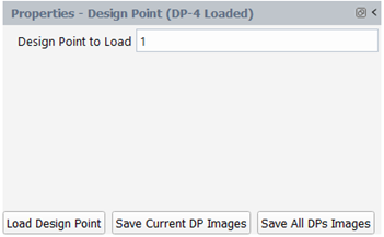
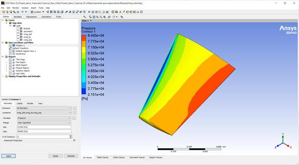
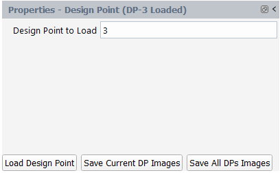
You will now go to the Design Point (DP-# Loaded) section. This section is used to visualize graphics results such as contours, vectors, pathlines, XY plots and scenes for a specific design point in the graphics window. After creating these graphics objects, you can easily replicate them for the remaining design points with a single click. From the Properties – Design Point (DP-# Loaded) panel,

Set Design Point to Load to 4
Click Load Design Point command to load the solution file of design point 4.
Go to Surfaces node to create lines located upstream of the wing tip to be used for creating pathlines in a later step.
Create a new line.
 Results → Design
Point → Surfaces
→ New → Line
Results → Design
Point → Surfaces
→ New → Line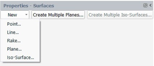
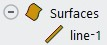
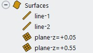
A line type object line-1 appears under Surfaces.
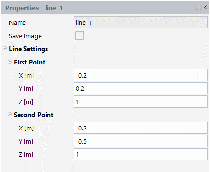
Set the following settings for line-1 in the Properties – line-1 panel.
In the First Point section:
Set X [m] to
-0.2.Set Y [m] to
0.2.Set Z [m] to
1.
In the Second Point section:
Set X [m] to
-0.2.Set Y [m] to
-0.5.Set Z [m] to
1.
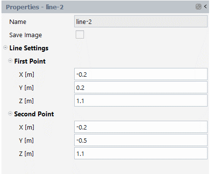
Create another new line. A line type object line-2 appears under surfaces. When creating line-2, follow the same steps as above using the settings in the following image.
Create two wing crossing planes which will be used to create contours.
Results → Design
Point → Surfaces
→ Create Multiple Planes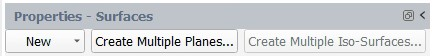
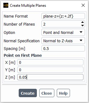
In the Create Multiple Planes dialog box:
Set Name Format to
plane-z={z:+.2f}.Set Number of Planes to
2.Set Option to Point and Normal.
Set Normal Specification to Normal to Z-Axis.
Set Spacing [m] to
0.5.In the Point on First Plane section:
→ Set X [m] to
0.→ Set Y [m] to
0.→ Set Z [m] to
0.05.When you're finished, click Create. Two planes now appear under Surfaces. The first plane is located near the wing root and the other closer to the mid span of the wing.
Select Contours under Graphics. There are two methods to create a contour. One way is to right-click on Contours, select New… and then specify the contour properties. Alternatively, you can predefine the properties from the Properties - Contours panel before creating the contour:
Results → Design
Point → Graphics
→ Contours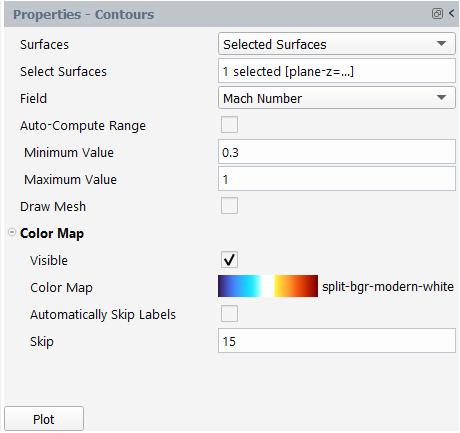
Set Surfaces to Selected Surfaces.
Set Select Surfaces to plane-z=+0.05.
Set Field to Mach Number.
Disable Auto-Compute Range.
Set Minimum Value and Maximum Value to
0.3and1respectively.In the Color Map section:
Enable Visible.
Set Color Map to split-bgr-modern-white.
Disable Automatically Skip Labels.
Set Skip to
15.
Click Plot to create and display the contour in the Graphics window. A contour-1 node now appears under Contours.

You will further adjust certain settings of contour-1. Select contour-1 under Contours and from the properties panel that appears:
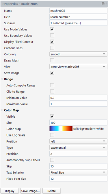
Change Name to mach-z005.
Enable the Save Image option to save the current contour image when executing the Save Current DP Images or Save All DPs Images command.
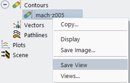
Go to the Graphics window and adjust the perspective view and position of the contour to your preference. From the Outline View, right click on mach-z005 and select Save View command. This will save the current view as aero-view-mach-z005 under the View option in the properties panel.
You can further adjust the remaining contour settings for mach-z005 in the properties panel. In the current example, we will keep the remaining settings on the properties panel.
Click Display to update the contour in the Graphics window.
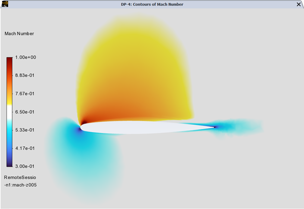
Note: The mesh used in this tutorial is very coarse. Its purpose is to quickly demonstrate a typical workflow in Fluent Aero and should not be relied upon for precise and/or accurate simulations. This mesh will not capture well viscous effects (such as viscous drag) or complex flow features (such as separation or wake).
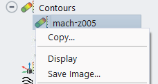
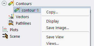
You will now use the Copy… function to create a contour of Mach number on plane-z=+0.55.
Right-click on contour mach-z005 and select Copy….
From the properties panel of the new contour that appears,
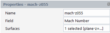
Change Name to mach-z055.
Set Surfaces to plane-z=+0.55.
Keep the remaining settings, including the View that you previously saved.
Click Display to show the contour in the Graphics window.
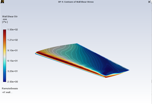
You will now create a contour of wall shear stress. Right-click on Contours and select New…. From the properties panel of the new contour that appears:
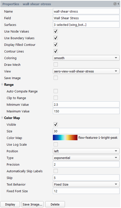
Change Name to wall-shear-stress.
Set Field to Wall Shear Stress which is under Wall Fluxes….
Select wing_bot, wing_te and wing_top for Surfaces.
Enable Use Node Values and Use Boundary Values.
Enable Display Filled Contour and Contour Lines.
Set Coloring to smooth.
Disable Draw Mesh.
Click Display to show the wall-shear stress contour.
Adjust the view from the Graphics window. Right-click on wall-shear-stress and then select Save View to save the view as aero-view-wall-shear-stress under View
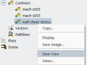
Enable Save Image option to save the current contour image when executing the Save Current DP Images or Save All DPs Images command.
In the Range section:
Disable Auto-Compute Range and Clip to Range.
Set Minimum Value and Maximum Value to
2.5and150respectively.
In the Color Map section:
Enable Visible.
Set Size to
30.Set Color Map to flow-features-1-bright-peak.
Disable Automatically Skip Labels.
Set Skip to
5.For the remaining settings, keep the default options.
Click Display to update the contour in the Graphics window.
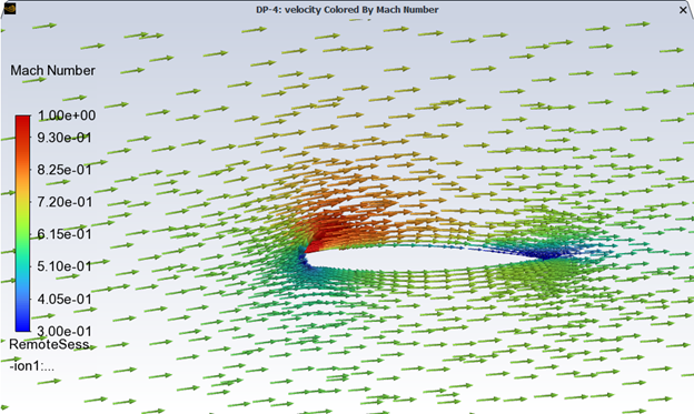
Create a vector plot.
Results → Design
Point → Graphics
→ Vectors New...
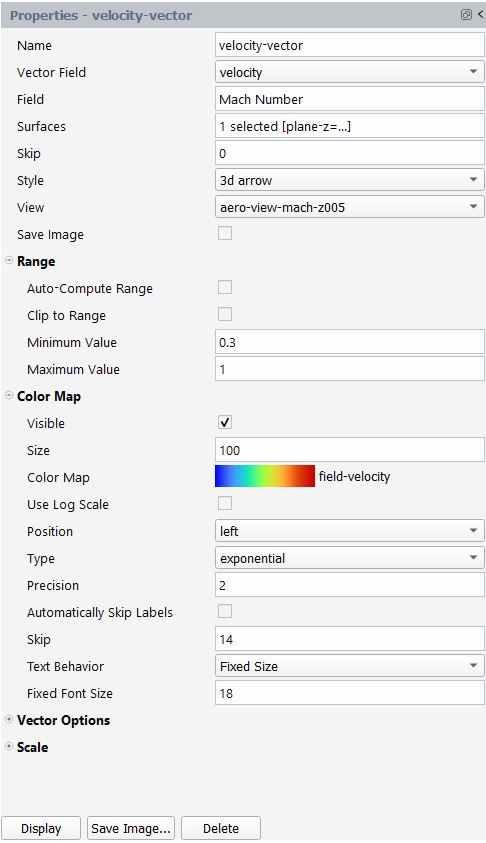
Set Name to velocity-vector.
Set Vector Field to velocity.
Set Field to Mach Number.
Set Surfaces to plane-z=+0.55.
Set View to aero-view-mach-z005.
In the Range section:
Disable Auto-Compute Range and Clip to Range.
Set Minimum Value and Maximum Value to
0.3and1respectively.
In the Color Map section:
Disable Automatically Skip Labels.
Set Skip to
14.Set Fixed Font Size to 18.
For the remaining settings, keep the default options.
Keep the default Vector Options and Scale options.
Click Display.
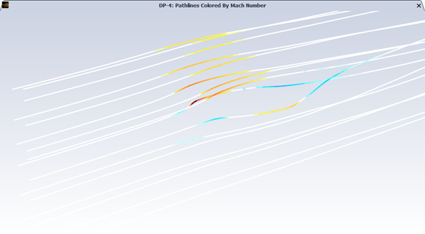
Create a pathline object to show the flow near the wing tip.
Results → Design
Point → Graphics
→ Pathlines New...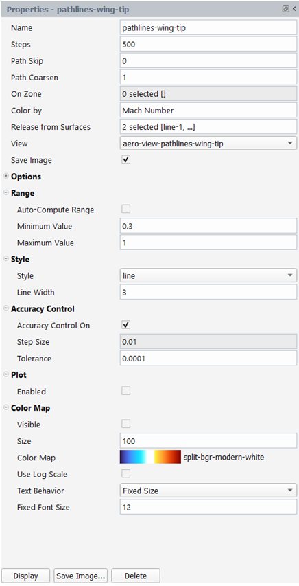
Set Name to pathlines-wing-tip.
Set Color by to Mach Number.
Set Release from Surfaces to line-1 and line-2.
Enable Save Image.
In the Range section:
Disable Auto-Compute Range.
Set Minimum Value and Maximum Value to
0.3and1respectively.
In the Style section:
Set Style to line.
Set Line Width to
3.
In the Accuracy Control section:
Enable Accuracy Control On.
Set Tolerance to
0.0001.
In the Color Map section:
Disable Visible.
Change Color Map to split-bgr-modern-white.
Keep all other settings to their default values.
Click Display. Keep in mind that the coarse mesh allows us to see only a few details in the complex wing tip flow.
Adjust the view for your plot of pathlines around the wing tip from the Graphics window.
Right click on pathlines-wing-tip from the Outline View and select the Save View command. The view will be saved as aero-view-pathlines-wing-tip under View.
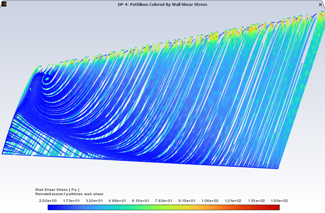
Create a pathline object to show the wall shear stress lines.
Results → Design
Point → Graphics
→ Pathlines New...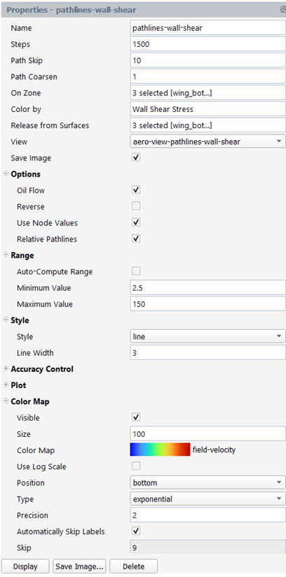
Set Name to pathlines-wall-shear.
Set Steps to 1500.
Set Path Skip to 10.
Under Options, enable Oil Flow.
Set On Zone to wing_bot, wing_te, and wing_top.
Set Color by to Wall Shear Stress.
Set Release from Surfaces to wing_bot, wing_te, and wing_top.
In the Range section:
Disable Auto-Compute Range.
Set Minimum Value and Maximum Value to
2.5and150respectively.
In the Style section:
Set Style to line.
Set Line Width to
3.
In the Color Map section, set Position to bottom.
Keep all other settings to their default values.
Click Display.
Adjust the view for your plot of pathlines on the wing surfaces from the Graphics window.
Right click on pathlines-wall-shear from the Outline View and select the Save View command. The view will be saved as aero-view-pathlines-wall-shear under View.
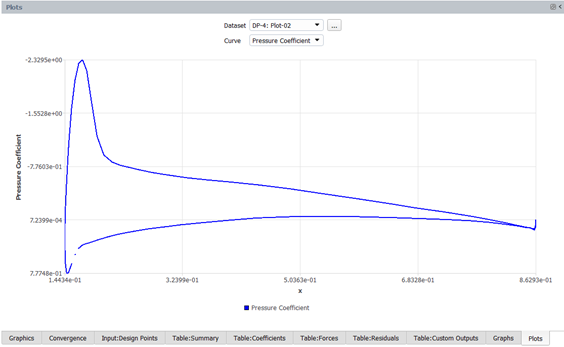
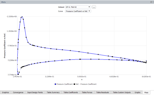
Click Design Point (DP-4 Loaded) → Plots in the Outline View. The Plots options can be used to quickly display simple 2D plots of selected design points and solution variables. The Properties - Plots window will be displayed.
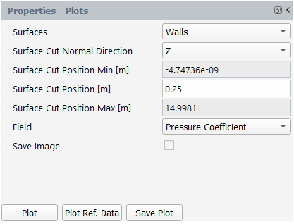
Set Surfaces to .
Set Surface Cut Normal Direction to .
Set Surface Cut Position [m] to
0.25.Set Field to .
Click .
The pressure coefficient on the walls of DP-4 at Z=0.25m will be plotted in the Plots window.
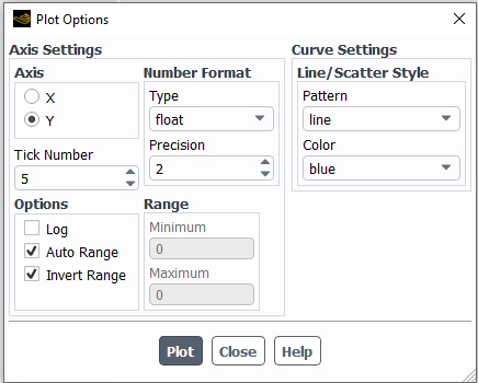
A Plot Options panel will appear after clicking the button. You can use this panel to customize plot settings for both axes. Press to apply these settings.
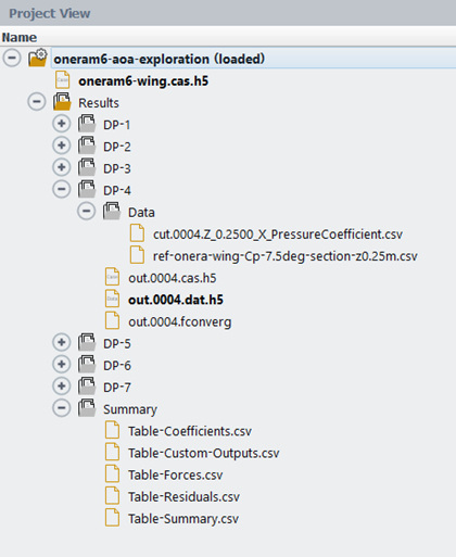
A .csv file will be saved in the Results folder after clicking the button, which is visible within the DP-4/Data folder in the Project View.
Click the button to load and plot a reference dataset in the current plot. In the dialog window that appears, browse to the reference file ref-onera-wing-Cp-7.5deg-section-0.25m.csv in the reference_data folder, and click . You can use the button to export the current plot to a .png file on disk. The reference data will be imported in the DP-4/Data folder in the Project View.
Figure 2.22: Data Folder in the Project View After Creating a Cut Plot and Plotting Reference Results
Create a scene object.
Results → Design
Point → Scene
New...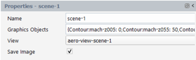
Open the Scene dialog box by pressing inside the Graphics Objects field. From the dialog box,
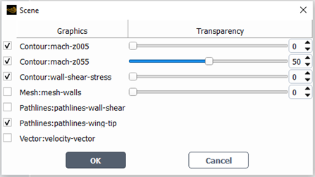
Enable Contour:mach-z005, Contour:mach-z055, Contour:wall-shear-stress and Pathlines:pathlines-wing-tip
Set Transparency of Contour:mach-z055 to 50.
Click OK to close the window.
Click Display and adjust the colormap positions and the view of your result figure.
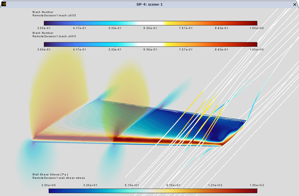
Right click on scene-1 from the Outline View and select the Save View command. The view will be saved as aero-view-scene-1 under View.
After generating all the graphics objects for design point 4, you can load a different design point and re-use these graphics objects. You also have the option to save the images of the graphics objects you created for the current design point or for all the updated design points.
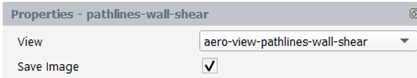
Navigate to the properties panel of the graphics objects that you want to save the image and activate the Save Image flag. You will check the Save Image option for pathlines-wall-shear among other results that you want to save.
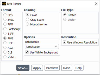
You can also click on the Save Image... button from the properties panel of a graphics object and customize the settings for saving your image. Click Apply to save these settings.
To save all graphics objects with the Save Image flag enabled for DP-4, click Save Current DP Images from the Properties – Design Point (DP-4 Loaded) panel. Fluent Aero will iterate over all the graphics objects with the Save Image flag activated and save the images in the Results folder.
To display the graphics objects for a different design point, change Design Point To Load to that design point and click Load Design Point. You can also load the results from the Project View by right-clicking on the solution file of the design point of interest and then selecting Load.
If you want to save images that have the Save Image option enabled for all the updated design points, click Save All DPs Images. The settings from the properties panel, including the specified view and save image options will be applied.
You will now create an animation using the images of pathlines-wall-shear saved in the previous step.
Click the New Animation from Files… button located in the Results -> Animation section of the ribbon.
In the Animation Options dialog box that appears, do the following:
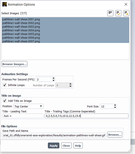
Navigate to the Results folder of the current simulation and select all the pathlines-wall-shear*.png files. The order in which you select the images determines the order in which they appear in the animation.
In the Animation Settings section:
Set Frames Per Second (FPS) to 2.
Enable Infinite Loops.
In the Title on Image section:
Enable Add Title on Image
Set Position to Top Center
Set Font Size to 12
Set Title -Leading Text to AoA =
Set Title – Trailing Tags (Comma-Separated) to 0,2.5,5.0,7.5,10.0,12.5,15.0.
Under File Options, specify the Save Pathand Name for your animation.
Click Apply to create and save the animation.
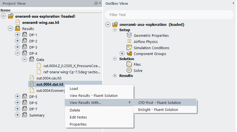
It is also possible to post-process Fluent Aero simulation results using an external post processing tool such as CFD-Post and EnSight. By right-clicking a .dat.h5 file in the Project View, a menu appears with several post-processing options such as and .
In this tutorial, you will use CFD-Post. Right-click out.0002.dat.h5 and select → to view the result file in CFD-Post. A CFD-Post window will appear where the data file can be further post-processed.
.
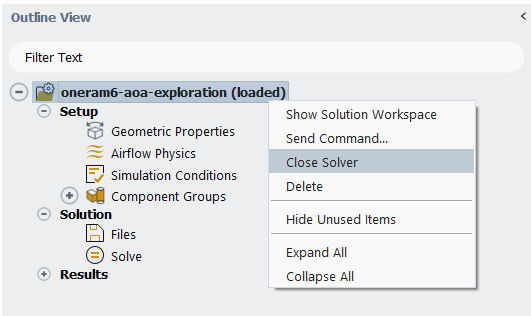
After completing the post-processing of the current simulation, right-click oneram6_aoa_exploration from the Outline View and then select . An information panel will appear to ask you if you want to save the case file or not. Click to save the case file.
If you would like to create a new simulation, select Simulation → from the Project ribbon. Browse and select a file to create a new simulation.
Once you have completed all your simulations, close the project and exit Fluent Aero by selecting Project → followed by File → .
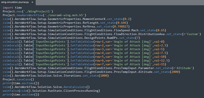
The objective of this part of the tutorial is to demonstrate the use of python journal scripting in Fluent Aero to complete the calculation of the design points. Specifically, this tutorial will demonstrate the following steps:
Recoding a python journal while setting up a simulation
Manually editing he python journal, including:
Adding additional Fluent Aero python commands
Adding external python modules commands
Executing the python journal (including using Fluent Aero in batch mode on a cluster)
Archiving the completed Fluent Aero project and deleting files to preserve disk space
In the following steps, we will record a python journal while setting up a base simulation using the Fluent Aero GUI.
For this tutorial, we will again use the oneram6-wing.msh.h5 file from the fluent_aero_tutorial.zip, from Part 1 of this tutorial, or – here .
Extract the
oneram6-wing.msh.h5file for this tutorial.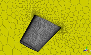
Launch Fluent 2024 R2 on your computer. On the Fluent Launcher panel, set the Capacity Level to Enterprise. Then select Aero. Set the number of Solver Processes to 4-8. Click Start.
From the dropdown menu, select File -> Start Journal… In the dialog, set the name for the journal file as wing-simulation-journal.py. Click OK. Any operation that you perform in Fluent Aero will now be recorded to this python journal file.
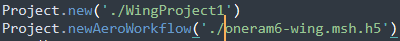
In the Project ribbon panel, select Project→New… and enter WingProject1 to create a new project folder.
In the Project ribbon, select Simulation→New Aero Workflow, and browse to and select the
oneram6-wing.msh.h5file. A New Simulation window will appear. Enter the Name of the New Simulation as oneram6-wing, and check Load in Solver. Click OK.In the Outline View window, click Geometric Properties.
Define the orientation of the geometry within the computational domain, which will be used to compute the aerodynamic forces.

Set the Moment Center X, Y and Z Position [m] to 0.2, 0, and 0, respectively.
Set the Reference Length [m] to 0.646, which corresponds to the mean chord length.
Set the Reference Area [m^2] to 0.748827.
In the Setup tree, go to Airflow Physics. A Properties – Airflow Physics window appears below the Outline View window.
In the Models section:
Set Knudsen Number Criterion to Disabled.
In the Setup tree, go to Simulation Conditions. In the Properties – Simulation Conditions window, go to Flight Conditions.
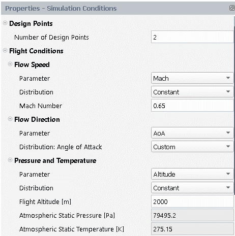
Set the Number of Design Points to 2
In the Flow Speed section,
Set the Mach Number to 0.65.
In the Flow Direction section,
Set Parameter to AoA.
Set Distribution: Angle of Attack to Custom.
In the Pressure and Temperature section,
Set Parameter to Altitude.
Set the Altitude [m] to 2000.
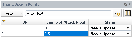
An Input:Design Points table will be created in the Graphics window on the right-hand side of the user interface.
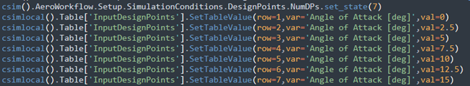
In the Angle of Attack [deg] column,
Set the Angle of Attack of DP 1 and 2 to 0 and 2.5, respectively.
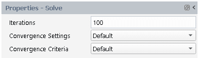
Under Solve, keep the default number of Iterations of 100. Keep both Convergence Settings and Convergence Criteria as Default.
Click the Update.
The calculation will start, and DP-1 and DP-2 will be calculated sequentially for 100 iterations.
Click the Update. The calculation will start, and DP-1 and DP-2 will be calculated sequentially, each with 10 iterations.
From the dropdown menu, select File -> Stop Journal to stop recording any more lines to the python journal.
In the following steps, we will use a tex editor to manually edit the python journal by adding additional Fluent Aero python commands and by including the use of an external python module.
Open the wing-simulation-journal.py that was recorded in a text editor, and view it’s contents. Take note that all of the operations performed in the above steps have been recorded to this journal.
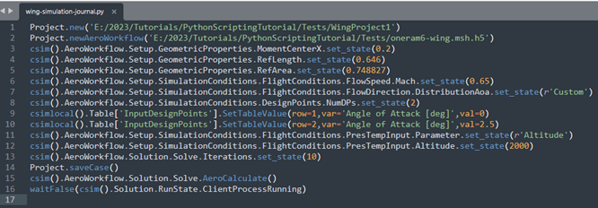
Our next objective will be to modify this journal with additional settings. Modify this file in the following ways.
Change the file paths associated with Project.new and Project.newAeroWorkflow so that they are relative paths. This will allow us to use these paths on other computers that don’t have the same directory structure.
Increase the Number of Design Points to 7, and define the Angle of Attack of each design point.
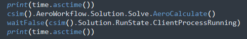
Increase the Number of Iterations to 1000, so sufficient iterations are performed for each design point.
Within the python script, it is also possible to import and use other python libraries. As an example, modify the script to add time printouts before and after the simulation, as follows
At the top of the file, import the time library
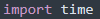
Before and after the AeroCalculate step (which is equivalent to the Update button in Fluent Aero), use the time library to print the time to the transcript.
Note: the time module is only used as an example. You can expand your usage of python modules to do any number of python operations during the execution of your script, including file management, post processing, and more.

After the above modifications, our script looks like this:
In the following steps we will copy our input mesh file and python journal file to a compute machine, and use them to launch Fluent Aero in batch mode and to execute the required python journal operations.
Create a directory on your compute machine or cluster called PythonScriptingTutorial. Copy the oneram6-wing.msh.h5 file and the wing-simulation-journal.py file to this directory on a compute cluster where you would like to run your full simulation.
Open a terminal and navigate to the PythonScriptingTutorial directory that contains your files.
Launch Fluent Aero using the aero executable in batch mode and read your python journal script using the following command.
/path/to/ansys_inc/v242/fluent/bin/aero -R wing-simulation-journal.py -N
where -R specifies the journal to be read, and -N specifies to run in batch mode.
(Optional) If using a compute cluster with a queuing system, you must include the proper job scheduler arguments required by your machine. One way to do this is to include the scheduler arguments in the launch command. In the example below, we are using a slurm cluster, and the command line has been extended using the scheduler arguments.
/path/to/ansys_inc/v242/fluent/bin/aero -R wing-simulation-journal.py -N -t28 -scheduler=slurm -scheduler_queue=partition-name -scheduler_account=account-name -scheduler_headnode=visualization-node-name
Note: In some instances, a cluster may require additional commands or a different approach to launch Fluent Aero. More information on these different approaches can be found in Launching Fluent Aero in Batch or on a Cluster using Job Scheduler.
Fluent Aero will launch in batch mode and read the wing-simulation-journal.py and execute the contents of the script. The console log of the actions performed by Fluent Aero should appear in the terminal. Once the python script has been fully executed, the Fluent Aero batch process will close.
Note: While the simulation is running in batch mode, do not open the project using the Fluent Aero UI. If you would like to view the results in the UI, please wait until the batch run has completed.
In the following steps, we will reduce the disk space used by the project by deleting unnecessary files, and subsequently archive the project using TAR.
After successful execution of the python script, two files will have been produced in the PythonScriptingTutorial directory: 1) a WingProject1.flprj file, which is an XML format file that contains information about all files associated with the project (location, dependencies, metadata) and 2) a WingProject1.cffdb folder, which contains all the files associated with the project.
Option 1 - creating an archive of the complete project:
If there are no disk space limitations, we can archive the complete project by creating a single tar file of these two items, using the following command:
tar -czvf WingProject1-Complete.tar.gz WingProject1.flprj WingProject1.cffdb
Notice that this creates an archive of the project with a size of about 400Mb.
Option 2 – deleting unnecessary case and solution files before archiving the project, to preserve disk space:
If there are disk space limitations, we can delete some case and solution files before archiving the project.
Some files should never be deleted, as they are required for the integrity of the Fluent Aero project (i.e. without them the Fluent Aero project and Simulation will not load correctly). These include:
The top level case file of a simulation (here: oneram6-wing/oneram6.cas.h5)
The run settings of a simulation (here: oneram6-wing/Results/run.settings)
However, some files are not required for Fluent Aero to load correctly, and one can consider the possibilyt of deleting them to preserver space. These include:
The design point case files (here: oneram6-wing/Results/out.000#.cas.h5). These files are only used to allow a user to repeat the design point calculation inside a classic Fluent solution environment – they are not required by Fluent Aero. We can safely remove these files to preserve space without affecting the usefulness of our Fluent Aero project.
The design point solution files (here: oneram6-wing/Results/out.000#.dat.h5). These files contain the full CFD solution of the design point, and can be used to do detailed investigation and post processing of the design point, including contour and image creation. If we still want to do detailed post processing and create contour images, we must keep these files. However, if we only require the automatically tabulated post processed results (like lift and drag coefficients), which are provide by the Table-*.csv files and the WingProject1.flrpj file, we could decide to delete these files to preserve space in our archive.
Because we used the default Files settings, inside the completed simulation results folder (WingProject1.cffdb/oneram6-wing/Results), we have design point case and solution files for each of the 7 design points (out.000#.cas.h5, out.000#.dat.h5).
While this is entirely depended on the specific requirements of the project, a good intermediate approach might be to keep the case and solution files for a single design point (to allow detailed post processing of at least one design point condition), and to remove the case and data files for all other design point (to preserve space in our archive).
Additionally, you have a few options for how you would like to remove these files. You could either completely delete the files from the folder and then create an archive (using the previous tar command), or you can exclude these files from the archive from within the tar command.
To exclude all design point case and data files except for design point 1 from the archive, use the following command:
tar -czvf WingProject1-Reduced.tar.gz –exclude=’out.000[!1]*.*.h5’ WingProject1.flprj WingProject1.cffdb
Notice that this creates an archive of the project with a size of about 75Mb (which is about 20% of the size of the archive of the complete project).
Note: there are numerous ways to perform this cleanup (manual deletion, scripted deletion, etc), and numerous tools that can be used to create the archive (tar, zip, etc). The important thing to take away from this tutorial section is that, depending on the user requirements, they can optionally remove design point case and solution files without affecting the integrity of the project.
Now that we have a neatly packaged archive of the project, we can transport this file to any computer required, and unpackage it at a later time to do additional calculations or post processing.
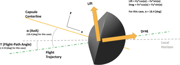
The main objective of this tutorial is to use Fluent Aero to compute the flow around an Earth re-entry capsule in a range of hypersonic flight conditions. The flight conditions used in this tutorial correspond to conditions experienced at different altitudes during an example flight path of a reference re-entry capsule, at altitudes ranging from approximately 50-70 [km] (Part I – Earth Re-Entry Simulation) and 80-92 [km] (Part II – Earth Re-Entry Simulation at High Altitudes). To improve accuracy, mixture representations of air are used in these simulations.
This tutorial also includes a demonstration case (Part III – Modeling the Flow Around an Entry Capsule in Martian Atmosphere) of a capsule entering the Mars atmosphere while considering air mixture properties and altitude conditions of the Martian atmosphere.
Note: In this tutorial, hypersonic flow conditions are simulated which make use of the
Two Temperature model for improved accuracy. This model is only
available with access to the cfd_hsf license increment and
the hsf library. If you attempt to run this tutorial
without this license increment or the hsf library, the
Two Temperature model will be and
the mixture representation of air cannot be used. Therefore, your results may differ
from what is shown here. If either the required license increment or the library are
unavailable, a message will be printed in your console log. Contact your Ansys
representative to add these resources if needed.
Part I – Earth Re-Entry Simulation
Download the fluent_aero_tutorial.zip file here .
Unzip fluent_aero_tutorial.zip to your working directory.
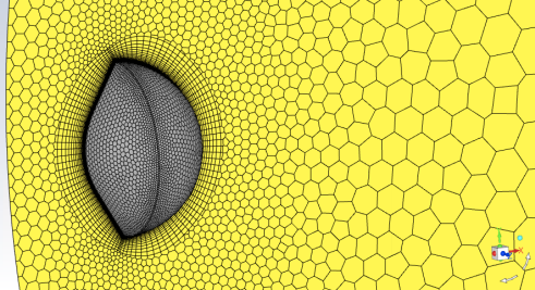
Extract the Capsule.msh.h5 file for this tutorial. The grid is an all-poly mesh which consists of 620,000 nodes and 180,000 cells. The limits of the computational domain are defined by a pressure-far-field, pressure-outlet, and a symmetry plane in the Z direction.
Launch Fluent 2024 R2 on your computer. On the Fluent Launcher panel that appears, set the Capacity Level to . Then select Aero. Set the number of Solver Processes to
4-16. Click .In the Fluent Aero workspace, go to the Project ribbon. Click Workspaces → , and make sure to uncheck , and .
When Fluent Aero first opens, the Project tab will be displayed by default. In the Project ribbon panel, select Project → and enter
Fluent_Aero_Tutorial_02to create a new project folder.In the Project’ ribbon, select Simulations → , and browse to and select the Capsule.msh.h5 file. A New Simulation window will appear. Enter the Name of the New Simulation as
Capsule_Custom_Exploration, and check .The case file will open and a background solver session will load. A new simulation folder will be created in your project folder. Fluent Aero will convert the .msh.h5 grid file to a .cas.h5 format case file and the latter will be imported in the simulation folder as Capsule.cas.h5.
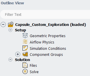
After the .cas.h5 file has been successfully loaded, a new Outline View tree appears under Capsule_Custom_Exploration (loaded).
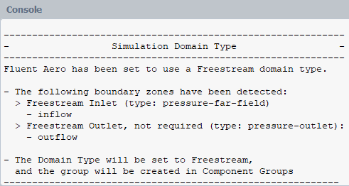
While importing, Fluent Aero will search for and find the pressure-far-field zone that defines the external boundary of the domain. Its presence will cause Fluent Aero to determine that this case is using a Freestream Domain Type, and the following message will be reported in the Console.
From the Outline View window, go to Geometric Properties. At the top of the Properties – Geometric Properties window, notice that the Domain Type has been automatically set to .
Define the orientation of the geometry within the computational domain. This is used to compute the aerodynamic forces.
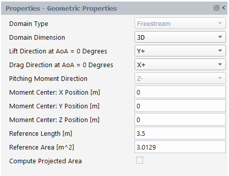
Set Domain Dimension to .
Set Lift Direction at AoA = 0 degree to .
Set Drag Direction at AoA = 0 degree to .
The Pitching Moment Direction will be automatically set to .
Set the Moment Center X-, Y- and Z-Position [m] to
0,0, and0, respectively.Set the Reference Length [m] to
3.5.Set the Reference Area [m^2] to
3.0129.
In the Setup tree, go to Airflow Physics. A Properties – Airflow Physics window appears below the Outline View window.
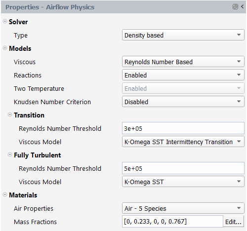
In the Solver section:
Set Type to .
In the Models section:
Set Viscous to .When selected, two sections, Transition and Fully Turbulent appear below, allowing you to define the Reynolds Number Threshold and Viscous Model to apply for each flow regime.
Set Reactions to . When enabled, you will be able to use a mixture representation of air in the next step and the Two Temperature model will be automatically set to .
Note: The Two-Temperature model is used to improve the accuracy of hypersonic flow simulations, like those used in this tutorial. It is only available if you have access to the
cfd_hsflicense increment and thehsflibrary. If you are unable to set the Two Temperature to , you may not have access to this license increment or thehsflibrary. Contact your Ansys representative to add these resources if needed.Set the Knudsen Number Criterion to .
In the Transition section:
Set the Reynolds Number Threshold that separates laminar and transition flows to 3e+05.
Set the Viscous Model for design points within the transition flow regime to K-Omega SST Intermittency Transition.
In the Fully Turbulent section:
Set the Reynolds Number Threshold that separates transition and fully turbulent flows to 5e+05.
Set the Viscous Model for design points within the fully turbulent flow regime to K-Omega SST.
In the Materials section:
Set the Air Properties to .
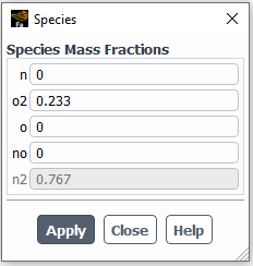
Set the Mass Fractions by clicking the button located on the right-hand side of the mass fractions display box to the species fractions shown below.
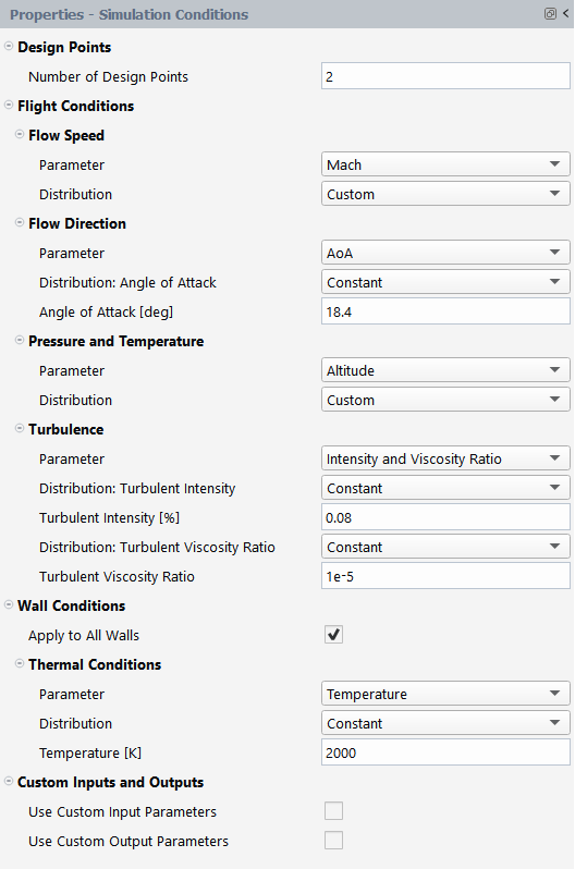
In the Setup tree, select Simulation Conditions. In the Properties – Simulation Conditions window.
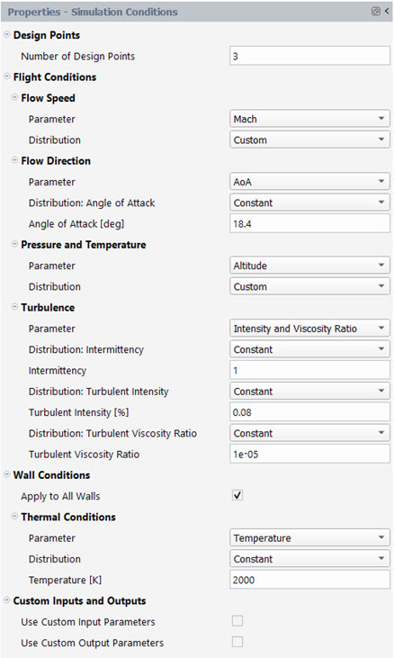
Set the Number of Design Points to
3.In the Flow Speed section,
Set Parameter to .
Set Distribution to .
For Flow Direction,
Set Parameter to .
Set Distribution: Angle of Attack to .
Set Angle of Attack [degrees] to
18.4.
In the Pressure and Temperature section,
Set Parameter to .
Set Distribution to .
In the Turbulence section,
Set Parameter to .
Set Distribution: Intermittency, Distribution: Turbulent Intensity and Distribution: Turbulent Viscosity Ratio to .
Set Intermittency to
1..Set Turbulent Intensity [%] to
0.08.Set Turbulent Viscosity Ratio to
1e-5.
In the Wall Conditions section:
Enable .
In the Thermal Conditions section:
Set Parameter to .
Set Distribution to .
Set Temperature [K] to
2000.
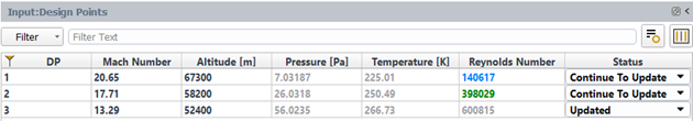
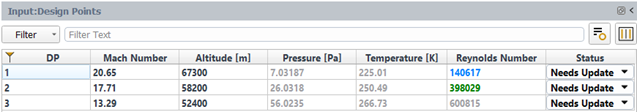
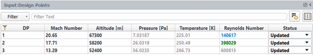
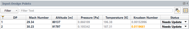
An empty Input:Design Points table will be created with 3 rows, one for each design point. You can manually fill the Input:Design Points table by clicking each entry cell and entering a value. Notice that there are 7 columns in the table. The first column specifies the Design Point number, and cannot be edited. The second and third columns are for specifying the variable inputs of Mach Number and Altitude [m], respectively. Since was selected under Pressure and Temperature, Pressure [Pa] and Temperature [K] are also shown in the table. These columns cannot be edited, as they will be automatically calculated and filled based on the Altitude input, which uses the International Standard Atmosphere. Since the Viscous Model is set to Reynolds Number Based, the next column shows the Reynolds Number. The final column lists the Status of each design point calculation.
Begin to manually fill the table by clicking the Mach Number cell of design point 1, and enter
20.65. Next, click the Altitude [m] cell and enter67300. Notice that the Pressure [Pa], Temperature [K] and Reynolds Numbercells are automatically filled with 7.0319, 225.01 and 140617, respectively. The Reynolds number value is highlighted in blue, indicating that the flow is in the laminar regime.Fill the remainder of the table by importing the data from a .csv file. Right-click the Simulation Conditions and select from the drop-down list of commands.
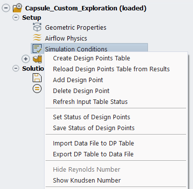
Navigate to and load the Capsule_Input_3_Design_Points.csv from the FLUENT_AERO_TUTORIALS folder and the remainder of the Input:Design Points Table will be filled.
You will notice that the Reynolds number values for the second and third design points are displayed in green and gray color, indicating that they are in the transition and fully turbulent flow regimes respectively.
Note: The Status of each design point (DP) is currently set to , because they have not yet been calculated.
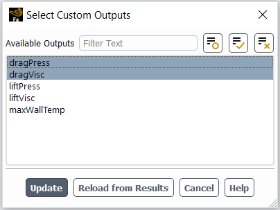
From the Properties - Simulation Conditions window, enable .
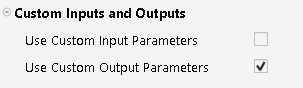
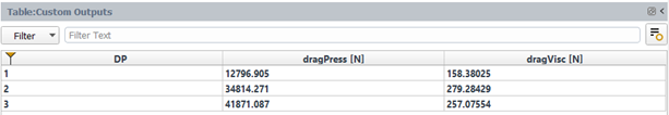
A selection panel will appear which contains a list of pre-defined custom-output variables. Select dragPress (pressure induced drag force), and dragVisc (wall shear stress induced drag force) and click . Fluent Aero will create the selected variables in the solver and the results of these output parameters will be shown in a table at the end of the calculation. Refer to Fluent Aero for more details about the functionality of the custom input/output parameters.
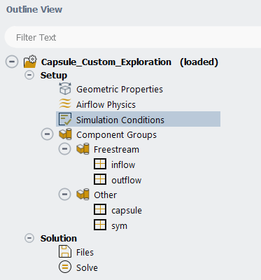
Go to Component Groups. Two default Component Groups have been created after the simulation is loaded. The Freestream group contains a pressure-far-field and a pressure-outlet zone that define the external boundary of the domain, and is where the freestream atmospheric flight conditions for each design point are defined as boundary conditions. The Other group contains the remainder of the boundary zones which are the walls of re-entry capsule and a symmetry plane of the simulation domain.
In the Outline View, go to Solution → Files. This step allows you to control the output files written per design point. Keep the default options.
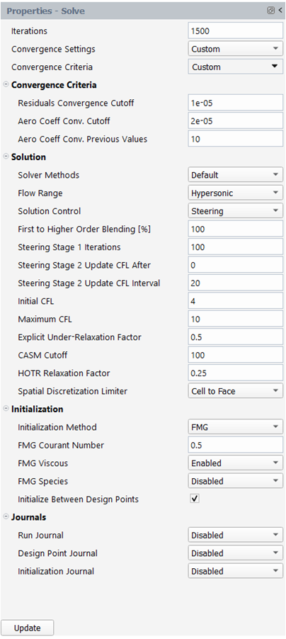
Under Solve, set the number of Iterations to
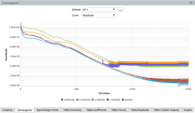
1500. Keep both Convergence Settings and Convergence Criteria as .Click the button at the bottom of the Properties - Solve panel. The simulation will first initialize using the flight conditions of DP-1 and then DP-1 will begin to iterate. The residuals plot of DP-1 will appear in the Convergence window located on the right of the screen.
In the Convergence window, set Dataset to and Curve to . The evolution of the drag coefficient for DP-1 will be displayed. You can query the value of the drag coefficient by left-clicking the curve.
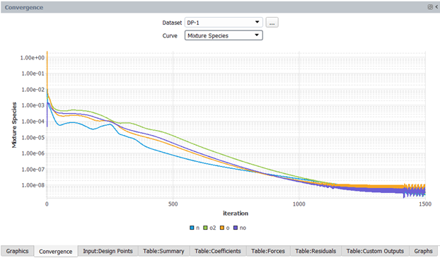
In the Convergence window, set Dataset to and Curve to . The residuals of species mass fractions for will be displayed. You can query the value of a specific species by left-clicking the curve.
After 1500 iterations, the DP-1 calculation is complete, the Status column in row 1 of the Input:Design Points table is set to , the results data file (.dat[.h5]) is saved, and the DP-2 calculation begins.
After all the design points have been updated, the status of the Input:Design Points table will be set to for all the design points.
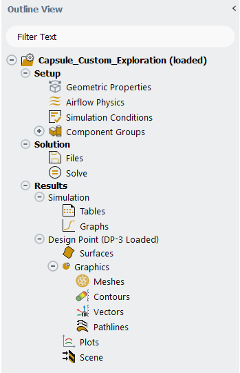
A Results node will be displayed in the Outline View after the simulation starts. This allows you to quickly postprocess all design point solutions, by obtaining aerodynamic coefficient plots, creating contour plots of solution fields, comparing solution fields to experimental data, and more.
Go to the Simulation node which provides a comprehensive view of aerodynamic coefficients across all design points. The first element in the Simulation node is Tables. In the current tutorial, five different Tables will be automatically created in the Graphics window area once the calculation is completed.
Note: You can also click Tables → button and the results tables will be exported to the Results folder of the current simulation and they will be visible in the Project View under the Summary folder.
Click the Table:Summary, Table:Coefficients, Table:Forces, Table:Residuals, and Table:Custom Outputs tabs at the bottom of the Graphics window to reveal each table.
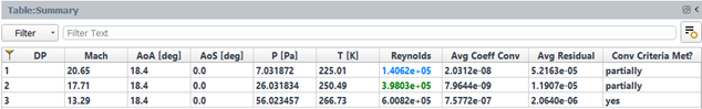
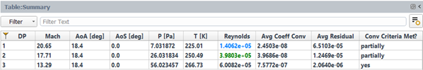
Table:Summary summarizes the flight conditions and convergence information for each design point.
Note: You can see from the convergence curves that lift and drag plateaued. However, you may notice in the final column of this table that all 3 design points have not fully met the default residuals convergence criteria of 1e-5. To have the Conv. Criteria Met? column set to , you could relax the convergence criteria by increasing the values of Residuals Convergence Cutoff or calculate for more iterations until the default convergence criteria is met. You can go to Solve, change Convergence Criteria to and Residuals Convergence Cutoff will be available within the Properties – Solve panel.
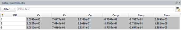
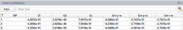
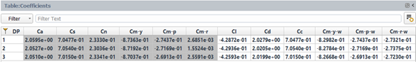
When the option is selected from the Display Aero Forces dropdown list in the Properties - Tables panel, Table:Coefficients contains the lift, drag, and moment coefficients. Moments are typically calculated in the , therefore, body-fixed axes moments, in addition to the lift and drag coefficients, which are coefficients, have been added to the default table. The body-fixed coefficients have been distinguished from the wind-fixed axes coefficients by the use of gray color. The final three columns show convergence data for the lift and drag coefficients, as well as the maximum convergence of the three moment coefficients.
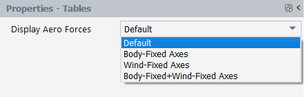
Fluent Aero currently supports the body-fixed and wind-fixed coordinate systems for displaying aerodynamic forces, moments, and coefficients. Display Aero Forces in the Properties - Tables panel allows you to display the forces and moments, as well as their coefficients, in the body-fixed, wind-fixed, or both coordinate systems at the same time. The images below demonstrate these options using the aerodynamic coefficients from this tutorial.
When is selected from Display Aero Forces in the Properties - Tables panel, Table:Forces contains the lift and drag forces, as well as the moment, as shown in Figure 2.37: Results Table of the Aerodynamic Forces when Default Is Selected. The gray color is used to differentiate between data from body-fixed axes and data from wind-fixed axes. Similar to Table:Coefficients, you can select from the same dropdown list to display forces and moments in either the body-fixed, wind-fixed, or both coordinate systems.
Note: When you right-click Tables in the Outline View and select , the displayed tables of forces and moments, along with their coefficients, will be written to Table-Coefficients.csv and Table-Forces.csv.
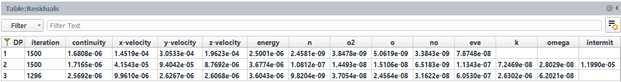
Table:Residuals summarizes the final residuals as well as the number of iterations run for each design point.
Table:Custom Outputs shows the final values of the custom outputs.
Click Graphs in the Outline View to show the plots of the aerodynamic coefficients defined in Fluent Aero. At the bottom of the Properties - Graphs window, click Plot Coefficients. An X-Y plot of lift coefficient () vs. design point (DP) will appear in the Graphics window. The drag and moment coefficients can be shown by selecting and from the Curve selection drop-down list.
You will now go to the Design Point (DP-# Loaded) section and visualize graphics results such as contours for a specific design point in the graphics window. After creating these graphics objects, you can easily re-use them for remaining design points. You will first analyze the graphics results for design point 3. From the Properties – Design Point (DP-# Loaded) panel,
Click Load Design Point command to load the solution file of design point 3.
Select Contours under Graphics. There are two methods to create a contour. One way is to right-click on Contours, select New… and then specify the contour properties. Alternatively, you can predefine the properties from the Properties - Contours panel before creating the contour:
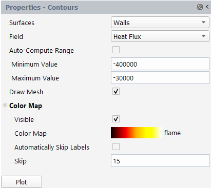
Set Surfaces to .
Set Field to .
Uncheck to disable .
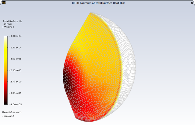
Set the Minimum and Maximum Value to
-400000and-30000respectively.Check to enable .
Click to expand Color Map.
Change Color Map to flame.
Uncheck and set Skip to
15.Click Plot to create and display the contour in the Graphics window. A contour-1 node now appears under Contours.

In the Graphics window, use the mouse to set the view of the contour. Right-click on contour-1 and then select Save View. This will save the current view as aero-view-contour-1 under the View option in the properties panel of contour-1.
Note: To change graphics display settings, you can go to File → → . For example, in the Lighting section, you can set Headlight to , and set appropriate values to both Headlight intensity and Ambient light intensity to personalize the graphics object rendering.
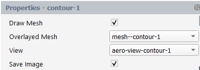
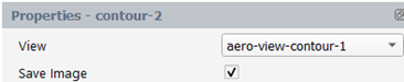
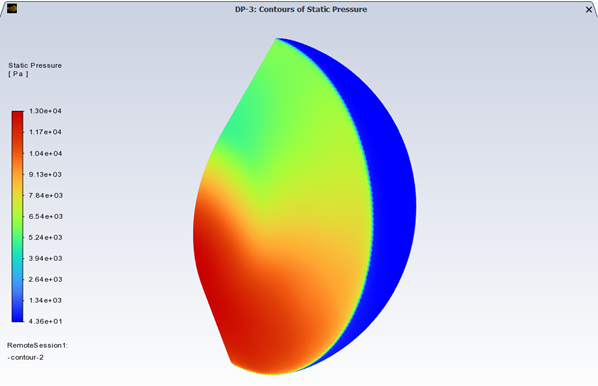
You will now create a contour of Static Pressure on wall surfaces. Right-click on Contours, select New…. A contour-2 node now appears under Contours. Go to the Properties – contour-2 panel:
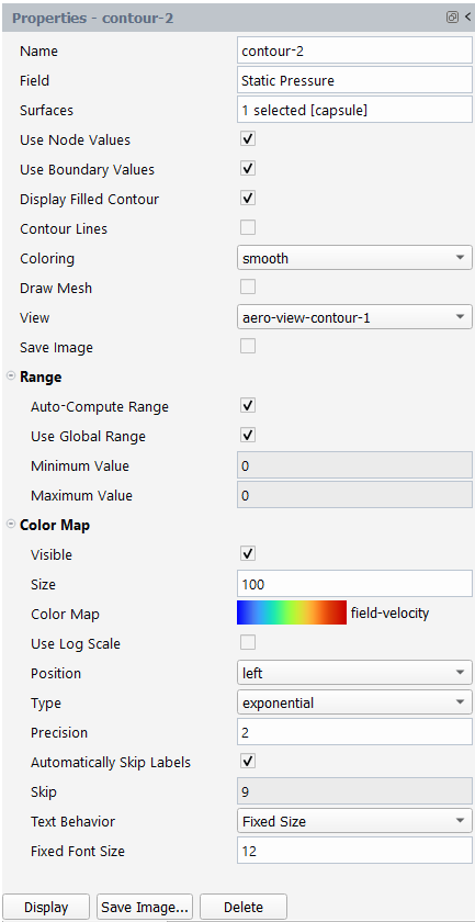
Set Field to Static Pressure.
Set Surfaces to capsule.
Set View to aero-view-contour-1.
Set Color Map to field-velocity.
For the remaining settings, keep the default options.
Click Display.
In this solution, notice the high pressure region around the stagnation point located towards the front of the capsule (left side in image), and the low pressure region in the backside of the capsule, which is surrounded by the wake.
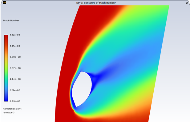
Click on Contours in the Outline View. In the Properties - Contours area, set Surfaces to Cutting Plane, Cutting Plane Normal Direction to Z, Cutting Plane Position [m] to
0.1and Field to Mach Number. Click to Enable Auto Compute Range. Click to Disable Draw Mesh. Set Color Map to Field Velocity. Click the Plot button to show the cutting plane contour in the Graphics window.Navigate to Design Point (DP-3 Loaded) → Plots. The Plots options can be used to quickly display simple 2D plots of selected design points and solution variables. The Properties - Plots window will be displayed.
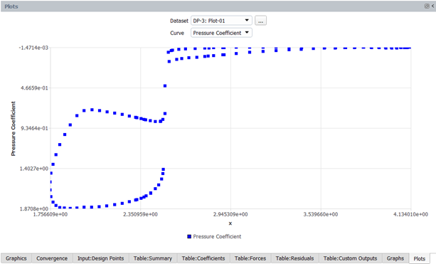
Set Surfaces to Walls.
Set Surface Cut Normal Direction to Z.
Set Surface Cut Position [m] to
0.1.Set Field to Pressure Coefficient.
Click Plot.
Since the solution for DP-3 at Z=0.1m will be plotted in the Plots window, a cut plot using default plot options will be created and a popup panel which allows you to customize certain plot options will appear. If the field is set to Pressure Coefficient, the Invert Range option for the y-axis will be enabled.
From the Plot Options panel, set the Pattern in Curve Settings to points-square. Click Plot. The 2D cut plot in the Graphics window will be updated using these new settings.
After generating all the graphics objects for design point 3, you can load a different design point and re-use these graphics objects. You also have the option to save the images of the graphics objects you created for the current design point or for all the updated design points.
Navigate to the properties panel of the graphics objects that you want to save the image and activate the Save Image flag.
You can also click on the Save Image... button from the properties panel and customize the settings for saving your image. Click Apply to save these settings.

To save all graphics objects with the Save Image flag enabled for DP-3, click Save Current DP Images from the Properties – Design Point (DP-3 Loaded) panel. Fluent Aero will iterate over all the graphics objects with the Save Image flag activated and save the images in the Results folder.
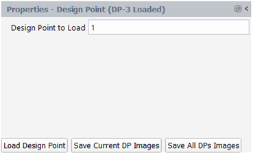
To display the graphics objects for a different design point, change Design Point To Load to that design point and click Load Design Point.
If you want to save images that have the Save Image option enabled for all the updated design points, click Save All DPs Images. The settings from the properties panel, including the specified view and save image options will be applied.
To further improve the convergence, you can continue to calculate the design points from the current results.
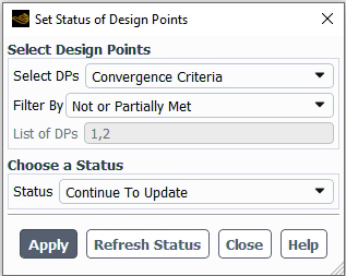
Go to the Input:Design Points table. Set the Status of design points that have not fully met the convergence criteria to . This operation can also be performed by using commands in the Design Points ribbon.
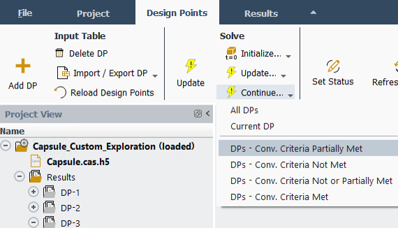
Click Design Points in the top ribbon.
Click Status → .
A Set Status of Design Points dialog opens which can be used to set the status of a group of design points.
Set Select DPs to .
Set Filter By to .
Set Choose a Status → Status to .
Click .
The status of all the design points will be set to .
In the Outline View, under Solution → Solve, set the Iterations to
250and click .Note: Other commands available in the Design Points ribbon can be useful to manage your calculation activities. For example, an alternative option to perform the procedure outlined above would be to use the Solve → command. This allows you to update a group of design points without needing to set their status. If you select and then select , all design points that have not met their convergence criteria will immediately .
Notice that after completing a calculation, the convergence of residuals have improved and the Conv. Criteria Met? of some design points might now be set to in Table:Summary.
Note: In the above tutorial, Fluent Aero’s default solver convergence settings are used to calculate the first 1500 iterations of each design point. However, in some cases, it is possible to start the calculation with different solver settings in order to improve convergence.
For example, you could repeat the above tutorial using more aggressive solver settings by performing the steps below.
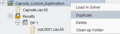
Create a simulation, set up the Geometric Properties, Airflow Physics and Simulation Conditions as previously described in the above steps. Alternatively, you can duplicate the previous simulation, including all setups, by right-clicking the Capsule_Custom_Exploration project folder located in the Outline View and selecting . You only need to change the solver settings.
In the Outline View, go to Solution → Solve. In the Properties - Solve panel, enter the following alternate settings:
Set the Iterations to
1500.Set Convergence Settings to . This will reveal additional options that can be useful to modify to attempt to improve the convergence or the speed of convergence.
Set the Convergence Criteria to . This will reveal the convergence cutoff values for residuals and aero coefficients, which can be modified to either improve or relax the convergence. Change the Flow Range from to . This will reveal solution steering settings.
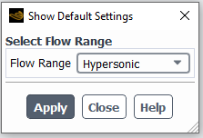
Right-click Solve from the Outline View and select the command.
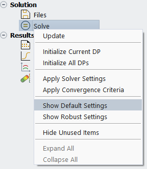
From the Show Default Settings panel, change Flow Range to and press . This will show the Convergence Settings set as that have been previously applied in the first part of this tutorial inside the Properties - Solve panel.
Increase the Initial Courant Number from
1to4.
Press to launch the calculation. With these more aggressive settings, the calculations will converge faster.
After completing the current simulation, you can close the solver by right-clicking Capsule_Custom_Exploration from the Outline View and selecting . An information panel will appear to ask you if you want to save the case file or not. Click to save the case file and preserve all the post-processing graphics settings.
Close the project and exit Fluent Aero. From the ribbon, select Project → to close a project. Next, select → and the Fluent Aero workspace will be closed.
Part II – Earth Re-Entry Simulation at High Altitudes
In this section, you will simulate a re-entry mission at high altitudes where flight conditions of a design point are in the transitional flow regime of rarefied gases. To enhance the accuracy of simulations at these conditions, an 11-species air mixture is used to account for ionization.
Open the project created in Part I – Earth Re-Entry Simulation.
In the Project ribbon, select Simulations → and browse to and select the Capsule.msh.h5 file. A New Simulation window will appear. Enter the Name of the New Simulation as
High_Altitude_ReEntryand check .Set the Geometry Properties as in Part I – Earth Re-Entry Simulation.
In the Setup tree, go to Airflow Physics. A Properties – Airflow Physics window appears below the Outline View window. Go to the → → Aero and enable . This will reveal the Transitional Regime Threshold above which the transitional regime for rarefied gases starts.
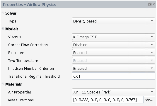
In the Solver section:
Set Type to .
In the Models section:
Set Viscous to .
Set Corner Flow Correction to Disabled
Set Reactions to . When enabled, you will be able to use a mixture representation of Earth's atmosphere in Materials and the Two Temperature model will be automatically set to .
Note: The Two Temperature model is used to improve accuracy of hypersonic flow simulations, like those used in this tutorial. It is only available if you have access to the
cfd_hsflicense increment and thehsflibrary. If you are unable to set the Two Temperature model to , you may not have access to this license increment or thehsflibrary. Contact your Ansys representative to add these resources if needed.Set Knudsen Number Criterion to .
Set Transitional Regime Threshold to
0.01.
In the Materials section:
Set Air Properties to .
Set Mass Fractions to
[0,
                                    0.233, 0, 0, 0, 0, 0, 0, 0, 0, 0.767]
by clicking the button located on the right-hand side of the mass fractions display box. Set the species fractions within the panel that appears.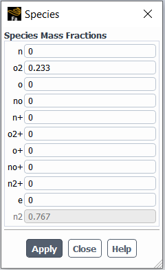
In the Setup tree, select Simulation Conditions. A Properties – Simulation Conditions window appears below the Outline View window.
Enter the Mach Number and Altitude [m] cells from DP-1 and DP-2 into the table, as shown in Figure 2.46: Input:Design Points Table of a Custom Exploration With 2 Design Points. When you enter the conditions for DP-2, a Knudsen Number column appears automatically because its Knudsen number is greater than the default threshold of 0.01 for the rarefied gas transitional flow regime. The orange color indicates that the Knudsen Number Criterion in Airflow Physics will be used for DP-2.
Keep the default settings in the Component Groups section.
Go to Solution → Files in the Outline View.
Keep the default settings.
Select Solve.
Set Convergence Settings to . Iterations automatically sets to
2000.Keep Convergence Criteria to .
Click the button. The simulation will begin with DP-1 and then progress to DP-2 once completed. The DP-1 residuals plot will appear in the Convergence window on the right side of the screen.
The convergence curves of the and groups will now be combined. In the Convergence window, select → → . You can now select and add curves to Curve → .
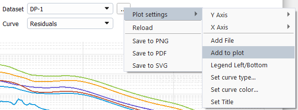
In the Add curve dialog, select under Add curve to plot and press . This will add all the species residuals under to .
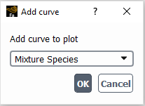
In the New curve dialog, under New curve name as
Residuals – Alland press .
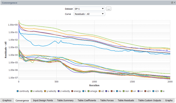
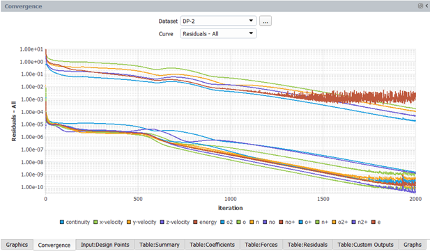
Set Dataset to in the Convergence window and repeat the steps to create the combined residuals plot for .
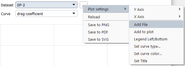
In the Convergence window, set Dataset to and Curve to . Select → → . This allows you to select a file and append its data to the current curves.
In the Open File dialog, navigate to and select out.0001.fconverg in the Results folder of the current simulation. On the second panel that appears, enter DP-1 as Tag for the new dataset.
You can now use the → → to combine the history of the drag coefficient from these two design points in the same plot.
In the Graphics window area, select Table:Summary where flight conditions and convergence information can be found. You can see from the convergence curves that the convergence of lift and drag plateaued. However, you may notice in the final column of this table that both design points have not fully met the default residuals convergence criteria of 1e-5. You could relax the convergence criteria by increasing the values of Residuals Convergence Cutoff to have the Conv. Criteria Met? column set to or run the calculations for more iterations until the default convergence criteria is met.
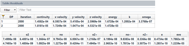
Select Table:Residuals to verify the final residuals as well as number of iterations run for each design point. Notice that the columns of k and omega are empty for DP-2 since laminar flow was imposed by the Knudsen Number Criterion.
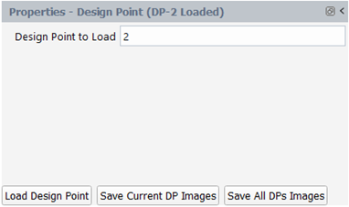
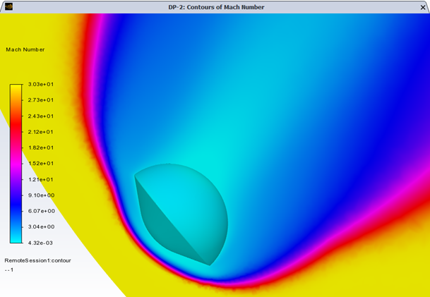
The Results node in the Outline View allows you to quickly post-process results by obtaining aerodynamic coefficient plots, creating contour plots of solution fields, comparing solution fields to experimental data, and more. For more information, refer to Part I – Earth Re-Entry Simulation. In this section, you will only generate contour plots of Mach number and molar concentration of electron. Go to Results -> Design Point (DP-# Loaded). From the properties panel, set Design Point to Load to 2 and click the Load Design Point button.
Left-click Contours from the Outline View to display the Properties – Contours window.
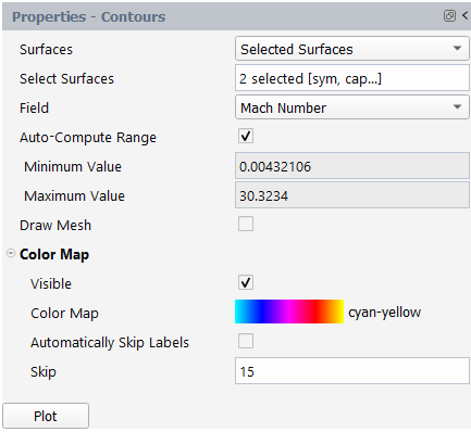
Set Surfaces to .
Set Selected Surfaces to sym and capsule.
Set Field to .
In the Color Map section:
Set Color Map to .
Uncheck and set Skip to
15.Click the button and adjust your view within the Graphics window.
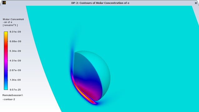
In the Properties – Contours panel, change only Field to . Click the button. Contours of the electron molar concentration will be displayed. The electron concentration is in the area behind the shock and the maximum electron molar density is 8.01e-9 kmol/m3, which is about 4.82e18 of electrons per cubic meter.
After completing the current simulation, you can close the solver by right-clicking High_Altitude_ReEntry from the Outline View and selecting . An Information dialog box will appear asking you to save the case file, click to save the case file and preserve all the post-processing graphics settings.
Part III – Modeling the Flow Around an Entry Capsule in Martian Atmosphere
In this section, you will simulate a Mars entry condition based on the flight path of the Viking lander mission 2 using the same capsule geometry as in Part I – Earth Re-Entry Simulation. In this case, to improve accuracy of simulations, the air mixture of the Martian atmosphere is used.
Open the project created in Part I – Earth Re-Entry Simulation.
In the Project’s ribbon, select Simulations → New Aero Workflow, and browse to and select the Capsule.msh.h5 file. A New Simulation window will appear. Enter the Name of the New Simulation as
Mars_Entry_Mission, and check .Set the Geometry Properties as in Part I – Earth Re-Entry Simulation.
In the Setup tree, go to Airflow Physics. A Properties – Airflow Physics window appears below the Outline View window. Go to the → → Aero and enable . This will reveal the Transitional Regime Threshold above which the transitional regime for rarefied gases starts.
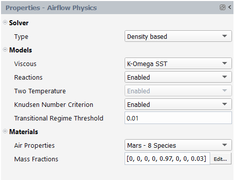
In the Solver section:
Set Type to .
In the Models section:
Set Viscous to .
Set Reactions to . When enabled, you will be able to use a mixture representation of the Martian atmosphere in Materials and the Two Temperature model will be automatically set to .
Note: The Two Temperature model is used to improve accuracy of hypersonic flow simulations, like those used in this tutorial. It is only available if you have access to the
cfd_hsflicense increment and thehsflibrary. If you are unable to set the Two Temperature model to , you may not have access to this license increment or thehsflibrary. Contact your Ansys representative to add these resources if needed.Set Knudsen Number Criterion to .
Set Transitional Regime Threshold to
0.01.
In the Materials section:
Set Air Properties to .
Set Mass Fractions to
[0, 0,
                                    0, 0, 0.97, 0, 0, 0.03]
by clicking the button located on the right-hand side of the mass fractions display box. Set the species fractions within the panel that appears.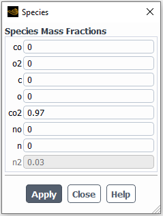
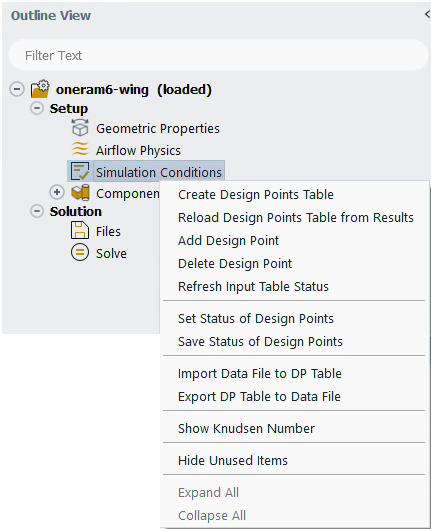
In the Setup tree, select Simulation Conditions. A Properties – Simulation Conditions window appears below the Outline View window.
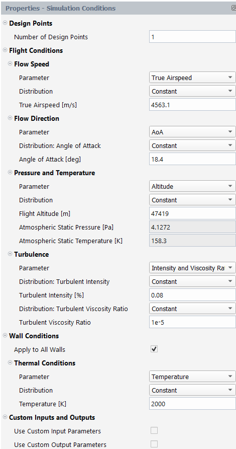
Set the Number of Design Points to
1.In the Flow Speed section:
Set Parameter to .
Set Distribution to .
Set True Airspeed [m/s] to
4563.1.
In the Flow Direction section:
Set Parameter to .
Set Distribution: Angle of Attack to .
Set Angle of Attack [deg] to
18.4.
In the Pressure and Temperature section:
Set Parameter to .
Set Distribution to .
Set Flight Altitude [m] to
47419. The Atmospheric Static Pressure [Pa] and Atmospheric Static Temperature [K] will be automatically computed based on the analytical altitude profiles created from the Viking lander re-entry profiles.
In the Turbulence section:
Set Parameter to .
Set both Distribution: Turbulent Intensity and Turbulent Viscosity to .
Set Turbulent Intensity [%] to
0.08.Set Turbulent Viscosity Ratio to
1e-5.
In the Wall Conditions section:
Enable .
In the Thermal Conditions section:
Set Parameter to .
Set Distribution to .
Set Temperature [K] to
2000.
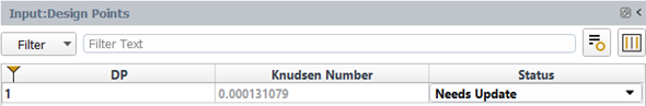
After setting the Simulation Conditions, Fluent Aero automatically calculates the Knudsen number (Kn). If any design point has a Knudsen number above the threshold of the transitional flow regime of rarefied gases, it will automatically be displayed in the input table. You can also manually show Knudsen number by right-clicking Simulation Conditions and selecting the . The Knudsen number of the current simulation is grayed out, indicating it is below the default threshold of 0.01 for the transitional regime. Consequently, the Knudsen Number Criterion that imposes laminar flow and partial slip wall conditions will not be applied to the current design point.
Keep the default Component Groups settings.
Go to Solution → Files in the Outline View.
Keep the default settings.
Select Solve.
Set Iterations to
1000.Keep Convergence Settings and Convergence Criteria to .
Click the button located at the bottom of the Properties - Solve panel. The simulation will first initialize using the flight conditions of DP-1 and then DP-1 will begin to iterate. The residuals plot of DP-1 will appear in the Convergence window located on the right of the screen.
In the Convergence window, set Dataset to and Curve to . The evolution of the drag coefficient for DP-1 will be displayed. You can query the value of the drag coefficient by left-clicking the curve.
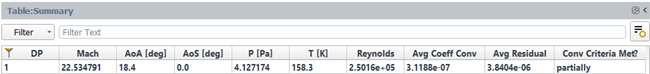
Go to the Graphics window area and select Table:Summary where flight conditions and convergence information can be found. You can see from the convergence curves that the convergence of lift and drag plateaued. However, you may notice in the final column of this table that DP-1 has not fully met the default residuals convergence criteria of 1e-5. You could relax the convergence criteria by increasing the values of Residuals Convergence Cutoff to have the Conv. Criteria Met? column set to or calculate for more iterations until the default convergence criteria is met.
The Results node in the Outline View allows you to quickly post-process results by obtaining aerodynamic coefficient plots, creating contour plots of solution fields, comparing solution fields to experimental data, and more. For more information, refer to Part I – Earth Re-Entry Simulation.
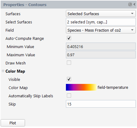
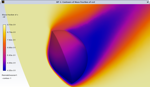
You will generate a contour plot of the CO2 mass fraction below. Left-click Contours from the Outline View to display the Properties – Contours window.
Set Surfaces to .
Set and as Selected Surfaces.
Set Field to .
Click to expand Color Map.
Set Color Map to .
Uncheck and set Skip to
15.Click the button. From the Graphics window, adjust the view.
After completing the current simulation, you can close the solver by right-clicking Mars_Entry_Mission from the Outline View and selecting . An Information dialog box will appear asking you to save the case file, click to save the case and preserve all the post-processing graphics settings.
Close the project and exit Fluent Aero by selecting Project → Close followed by → to close the Fluent Aero workspace.
The objective of this tutorial is to introduce the aircraft Component Groups feature in Fluent Aero and to compute the flow around a common commercial aircraft at different flight Altitudes, Mach and engine regimes. The aircraft considered is the NASA Common Research Model (CRM) in the wing-body-nacelle-pylon (WBNP) configuration. The flight conditions used in this tutorial represent examples of climb and nominal cruise conditions and are for demonstration purposes only.
Download the fluent_aero_tutorial.zip file here .
Unzip fluent_aero_tutorial.zip to your working directory.
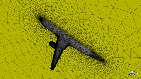
Extract the CRM_WBNP_Aircraft.msh.h5 file for this tutorial. The grid consists of 1.2M nodes and 2.4M cells. Five layers of prisms are grown off the aircraft’s wall boundaries and the remainder of the computational domain is filled with tetrahedral cells. The limits of the computational domain are defined by a hemispherical boundary defined as a pressure-farfield boundary type, and a flat circular boundary defined as a symmetry plane in the Z direction. This .msh file therefore meets the General Case File or Mesh File Requirements. However, the mesh is very coarse, and therefore should be used for demonstration purposes only.
Launch Fluent on your computer. On the Fluent Launcher panel that appears, set the Capacity Level to . Then select Aero. Set the number of Solver Processes to
4-8. Click .In the Fluent Aero workspace, go to → . In the Preferences window, go to the Aero menu and ensure Use Custom Solver Launch Settings, and are disabled. Disabling these settings is the preferred approach for running Fluent Aero simulations on your local machine.
When Fluent Aero first opens, the Project tab will be displayed by default. In the Project ribbon panel, select Project → and enter
Fluent_Aero_Tutorial_03to create a new project folder.In the Project ribbon, select Simulation → , and browse to and select the CRM_WBNP_Aircraft.msh.h5 file. A New Simulation window will appear. Enter the Name of the New Simulation as
CRM_WBNP_Aircraft, and check .The case file will open and a background solver session will load. A new simulation folder will be created in your project folder. Fluent Aero will convert the .msh.h5 grid file to a .cas.h5 format case file and the latter will be imported in the simulation folder as CRM_WBNP_Aircraft.cas.h5.
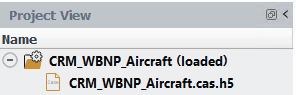
After the case file has been successfully loaded, a new Setup tree appears under CRM_WBNP_Aircraft (loaded) in the Outline View window.
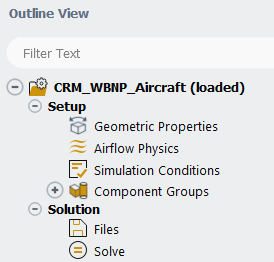
While importing, Fluent Aero will search for and find the pressure-far-field zone that defines the external boundary of the domain. Its presence will cause Fluent Aero to determine that this case is using a domain type, and the following message will be reported in the Console.
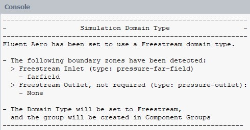
In the Outline View window, under the Setup tree, go to Geometric Properties. A Properties – Geometric Properties window appears below the Outline View. Define the orientation of the geometry within the computational domain, which is used to compute the aerodynamic forces.
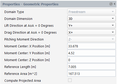
Set Domain Dimension to .
Set Lift Direction at AoA = 0 degree to .
Set Drag Direction at AoA = 0 degree to .
Set the Moment Center X-, Y- and Z-Position [m] to
33.678,4.520, and0, respectively.Set the Reference Length [m] to
7.005.Set the Reference Area [m^2] to
167.513which is the reference wing area.Alternatively, you can use to calculate the reference area.
Enable .
From the Projected Surface Areas panel
Set Projection Direction to .
Keep Min Feature Size [m] as
0.001.In the Walls section, select all walls staring with wing-.
Press . The reference wing area will be computed and displayed.
Press to use the computed area as the Reference Area [m^2] in the Properties – Geometric Properties panel.
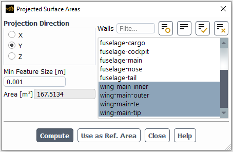
In the Setup tree, go to Airflow Physics.
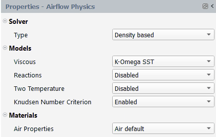
In the Solver section:
Set Type to .
In the Models section:
Set Viscous to .
Set Reactions to .
Set Two Temperature to .
Set Knudsen Number Criterion to .
In the Materials section:
Set Air Properties to .
You will now set up the Freestream flight conditions. Two design points will be created. The first DP represents an example of a climb condition and the second DP corresponds to a nominal cruise condition and they are for demonstration purposes only. In the Setup tree, go to Simulation Conditions. In the Properties – Simulation Conditions window,
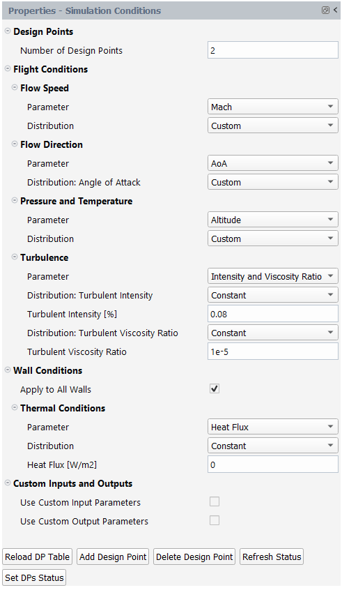
Set the Number of Design Points to
2In the Flow Speed section,
Set Parameter to .
Set Distribution to . An empty column will appear in the Input: Design Points table where you can set the Mach Number for each design point.
In the Flow Direction section,
Set Parameter to .
Set Distribution: Angle of Attack to An empty column will appear in the Input: Design Points table where you can set the Angle of Attack for each design point. You will enter these conditions in the next step.
In the Pressure and Temperature section,
Set Parameter to .
Set Distribution to . An empty column will appear in the Input: Design Points table where you can set the Altitude for each design point.
Fill the Mach Number, Angle of Attack [deg] and Altitude [m] columns with the values shown below. The Pressure [Pa] and Temperature [K] columns will be automatically computed from the International Standard Atmosphere model at the altitude of each design point.
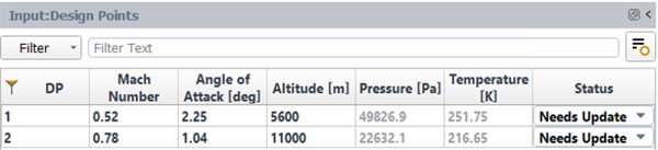
In the Turbulence section,
Set Parameter to .
Set both Distribution: Turbulent Intensity and Turbulent Viscosity to .
Set Turbulent Intensity [%] to
0.08.Set Turbulent Viscosity Ratio to
1e-5.
In the Wall Conditions section:
Enable .
In the Thermal Conditions section:
Set Parameter to .
Set Distribution to .
Set Heat Flux [W/m2] to
0.
You will now create several aircraft components which will allow you to define some component specific inputs and outputs. In the Setup tree, go to Component Groups. In the Properties – Component Groups window, click . The Component Manager panel will appear.
Use the Component Manager to create an type component:
In the New Component section, set Type to and a default group name Engine_01 will appear.
Use to add into Existing Components.
All the boundary zones that have not been assigned to any group are listed under Available Zones. An Engine type group is a specific type of group which contains three different Component Parts:
Exhaust
Intake
Nacelle
At least one boundary zone must be added to the Exhaust and Intake Component Parts.
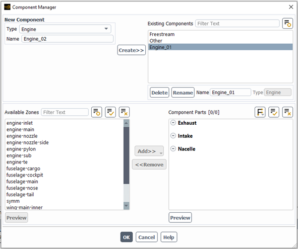
From Available Zones, select engine-inlet and use the button to add it to the Intake component part.
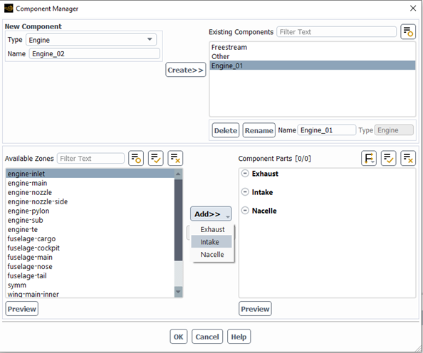
Select and add engine-nozzle to the Exhaust part.
Select and add all the remaining boundary zones starting with engine- to the Nacelle part.
The Engine_01 component group is now successfully created.
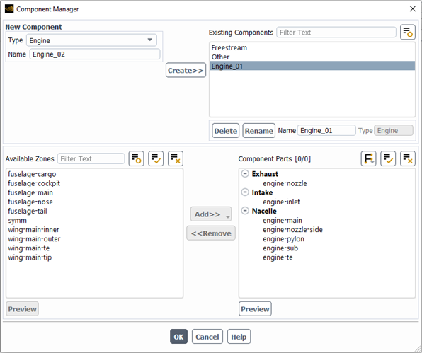
Use the Component Manager to create a Wing type component:
From the New Component section, change Type to .
Use to add Wing_01 to the Existing Components.
From Available Zones, select all the boundary zones that start with wing and use to add them to the Walls component parts.
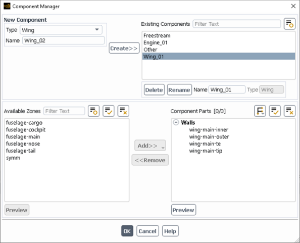
Use the Component Manager to create a General type component:
Change Type in the New Component to .
Change Name to
Fuselage.Use to add the Fuselage group to Existing Components.
From the Available Zones, select all the boundary zones with the fuselage- prefix and use to add them to the All component part.
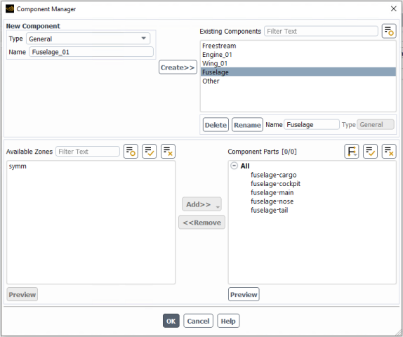
Click to close the Component Manager. The three new Component Groups will appear in the Outline View in addition to the default Freestream and Other groups.
From Outline View → Component Groups, expand the Engine_01 component and select engine-inlet which is a pressure-outlet type boundary zone. You will now set up the engine conditions.

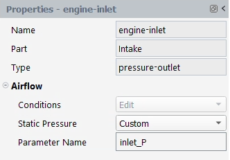
In the Properties – engine-inlet window:
Change Conditions to .
Set Static Pressure to to apply different Static Pressure [Pa] for each design point.
Change the default Parameter Name to
inlet_P.
A custom expression for the Static Pressure [Pa] will be created in the solution workspace with the name inlet_P. A column named inlet_P [Pa] will be added to the Input:Design Points table. You will enter the values of inlet_P [Pa] in a later step.
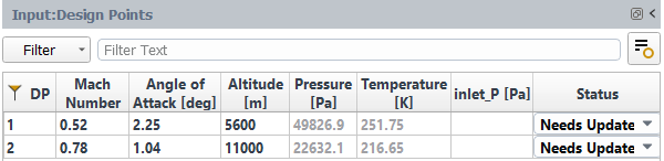
Select engine-nozzle to set boundary conditions at the engine exhaust.
Note: The engine exhaust surface in this tutorial is a single flat circular disk that accounts for the fan and the core airflow and therefore cannot well represent the double-flow design of a typical aircraft engine. In this manner, the engine thrust computed in the current tutorial is for demonstration purposes only.
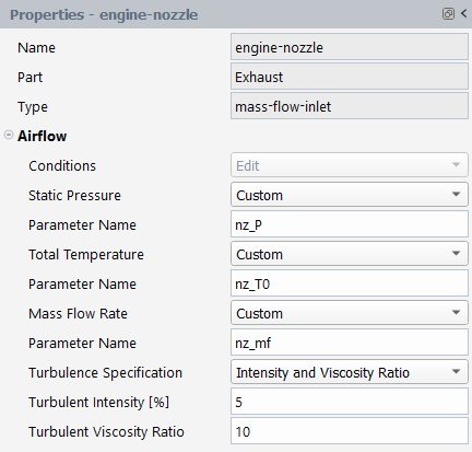
In the Properties – engine-nozzle window:
Change Conditions to .
Change Static Pressure, Total Temperature and Mass Flow Rate to to apply different Static Pressure [Pa], Total Temperature [K] and Mass Flow [kg/s] for each design point.
Change the default parameter names to
nz_P,nz_T0andnz_mfrespectively. Three custom expressions will be created in the solution workspace and will appear in the Input:Design Points table. Fill the table with the values as shown below.Keep the default turbulence settings.
Notice that there are 2 design points and 11 columns in the table. The first and second design points represent an example of climb and nominal cruise conditions respectively. Their flight conditions are provided for demonstration purposes only. The first column specifies the design point number and cannot be edited. The second to fourth columns contain the Mach Number, Angle of Attack [deg] and Altitude [m] and can be edited since these are custom parameters. Pressure [Pa] and Temperature [K] columns cannot be edited, as they will be automatically calculated from Altitude [m]. The next four columns define the boundary conditions of the Engine_01 group. They allow you to input conditions corresponding to different engine regimes. The last column is set to for both design points since they have not yet been calculated.
Next, enable additional output variables relevant to your components.
In the Setup tree, go to Component Groups.
In the Properties – Component Groups window:
Click the button to enable component specific output parameters.
From the Manage Component Outputs panel:
Check the box of the , Fuselage, Wing_01 and Engine_01 components.
Check the box of the Wing_01 component.
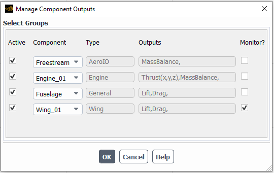
Because Active is enabled, the mass flow balance of the group, the lift and drag forces of the and components as well as the thrust and mass flow balance of will be calculated and summarized in Table:Component Outputs when the calculation terminates. Since Monitor? is enabled, the evolution of the Lift and Drag outputs will be plotted in the Convergence plot.
Click to close this panel.
Go to Solution → Files in the Outline View. This step allows you to control the output files that are written per design point. Keep the default options.
Go to Solution → Solve.
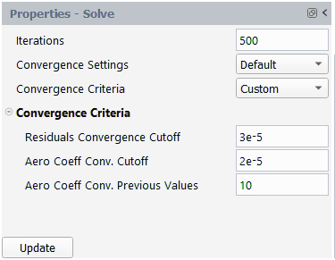
Set Iterations to
500.Keep Convergence Settings to .
Set Convergence Criteria to .
Set Residuals Convergence Cutoff to
3e-5.Set Aero Coeff Conv. Cutoff to
2e-5.Keep Aero Coeff Conv. Previous Values as
10.
Click the button at the bottom of the Properties - Solve panel.
The calculation will start, and the first design point, DP-1 will be simulated. A Convergence window will appear in place of the Graphics window and display the residuals and monitors for DP-1.
Design point DP-1 will run until the total number of Iterations (500) or the Residuals Convergence Cutoff (3e-5) and Aero Coeff Conv. Cutoff (2e-5) values have been satisfied, whichever comes first.
Look at the convergence history of the simulation in the Convergence window on the right of your screen. Set Dataset to and the Curve to to view the continuity, x-, y-, z-velocity, energy, and turbulence residuals for the first design point. You can left-click a residual curve to show the iteration number and the corresponding residual value. The residual of x-velocity at iteration 392 is shown and equals to 2.9389e-5 which is below the Residuals Convergence Cutoff (3e-5). The remaining residuals of the DP- 1 have also met the Residuals Convergence Cutoff criteria.
In the Convergence window, set Curve to . The evolution of the lift force on Wing_01 for DP-1 will be displayed. Left-click the last iteration of the lift-force plot, to show the value of the lift at the last iteration.
When the calculation of DP-1 is complete, the status column in row 1 of the Input:Design Points table will be set to , and the calculation of DP-2 will begin.
After all the design points have been updated, the status of the Input:Design Points table will be set to for all the design points.
A Results node will be displayed in the Outline View tree after the simulation starts. The Results node contains a Simulation and a Design Point sub-components. This allows you to quickly post-process all design point solutions, by obtaining aerodynamic coefficient plots, creating contour plots of solution fields, comparing solution fields to experimental data, and more.
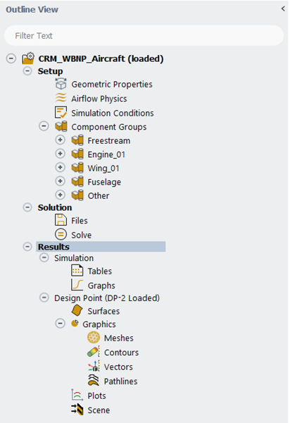
Go to Simulation node which provides a comprehensive view of aerodynamic coefficients across all design points. The first element in the Simulation node is Tables. In the current tutorial, five different Tables will be automatically created in the Graphics window area when the calculation is complete.
Click the Table:Summary, Table:Coefficients, Table:Forces, Table:Residuals and Table:Component Outputs tabs at the bottom of the Graphics window to reveal each table.
Table:Summary summarizes the flight conditions and convergence information for each design point. In the current simulation, although both design points have met the convergence criteria () as shown in the Conv. Criteria Met? column, it is still recommended to investigate your solutions to ensure that appropriate convergence levels have been achieved.
Table:Residuals summarizes the final residuals as well as the number of iterations run for each design point. For each design point, all residuals have met the Residuals Convergence Cutoff criteria.
Table:Coefficients contains the lift and drag calculated in the wind-fixed coordinate systems and moment coefficients calculated in the body-fixed coordinate systems which are highlighted in gray. The last three columns (Cl Conv., Cd Conv., Max Cm Conv.) show information related to the convergence of lift and drag coefficients and the maximum value among the three moment coefficients.
Note: While all residuals and convergence of the aerodynamic coefficients meet the convergence cutoff criterion of 3e-5 and 2e-5, it is still recommended for you to investigate your solutions to ensure that appropriate convergence levels have been achieved and that convergence remains stable. The default convergence cutoff criteria may be appropriate for some cases, but not for others, and therefore care should be taken when selecting this value.
Table:Forces contains the dimensional forces of lift, drag and moment. Similar to the results in Tables: Coefficients, lift and drag forces are computed in the wind-fixed coordinate system while moment forces are calculated in the body-fixed coordinate system.
Table:Component Outputs contains the lift and drag of the wing and fuselage groups, the mass flow balance of the freestream and engine groups and the thrust of the engine group.
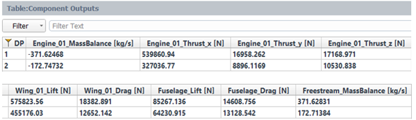
Click Graphs in the Outline View to show the plots of the aerodynamic coefficients defined in Fluent Aero.
At the bottom of the Properties - Graphs window, click Plot Coefficients. An X- Y plot of lift coefficient () vs. design point () will appear in the Graphics window.
The drag and moment coefficients can be shown by selecting and from the Curve selection drop-down list.
Select / from the Curve to show the lift to drag ratio as a function of the design point.
Click the button. An X-Y plot of Lift Coefficient (Cl) vs. Drag Coefficient (Cd) will appear in the Graphics window. Alternatively, you can simply change Dataset to from the Graphics window to show the drag polar plot.
You will now go to the Design Point (DP-# Loaded) section and visualize graphics results such as contours for a specific design point in the graphics window. After creating these graphics objects, you can easily re-use them for a different design point. From the Properties – Design Point (DP-# Loaded) panel,
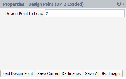
Set Design Point to Load to 2.
Click Load Design Point command to load the solution file of design point 2.
The Contours options under Graphics can be used to quickly display simple contour plots of selected design points and solution variables.
Left-click Contours from Outline View to display the Properties - Contours window.
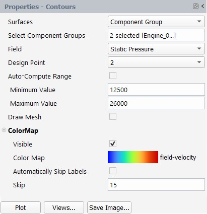
Set Surfaces to .
For Select Component Groups, select both the and groups.
Set Field to .
Uncheck the option.
Set the Minimum and Maximum Value to
12500and26000respectively.In the ColorMap section, uncheck , set Skip to
15and set Color Map to field-velocity.Click the button to create and display the contour in the Graphics window. A contour-1 node now appears under Contours.

You will further adjust certain settings of contour-1 from its properties panel that appears.
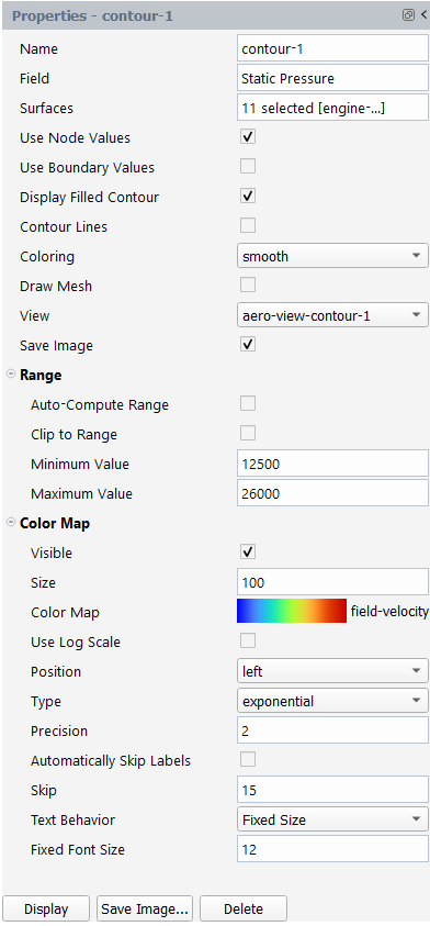
Enable the Save Image option to save the current contour image when executing the Save Current DP Images or Save All DPs Images command.
Go to the Graphics window and adjust the contour view to your preference. From the Outline View, right click on contour-1 and select Save View command. This will save the current view as aero-view-contour-1 under the View option in the properties panel.
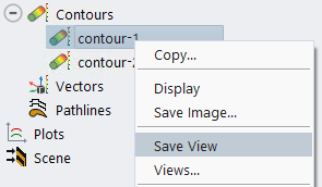
Click Display to update the contour in the Graphics window.
The selected contour will be displayed in the Graphics window where you can use the mouse to set the view of the contour. As you can see from the contour, some of the common flow features are captured. Due to the flow on the suction side between the fuselage and the nacelle, a strong flow acceleration is present. Flow encounters adverse pressure gradient moving downstream to the trailing edge. At the wing tip, the pressure is higher on the outer region than on the inner region which indicates the presence of transverse flow.
Note: The mesh used in this tutorial is very coarse. Its purpose is to quickly demonstrate a typical workflow in Fluent Aero and should not be relied upon for accurate simulations. For instance, this mesh may not capture well viscous effects (such as boundary layer and viscous forces) or complex flow features (such as flow separation). This should be considered while you investigate the solutions. For more accurate simulations, a finer mesh appropriate for external aerodynamic simulations, featuring more prism layers, higher mesh surface refinement, and increased mesh density in the wake region, should be used.
In the Properties - Contours area,
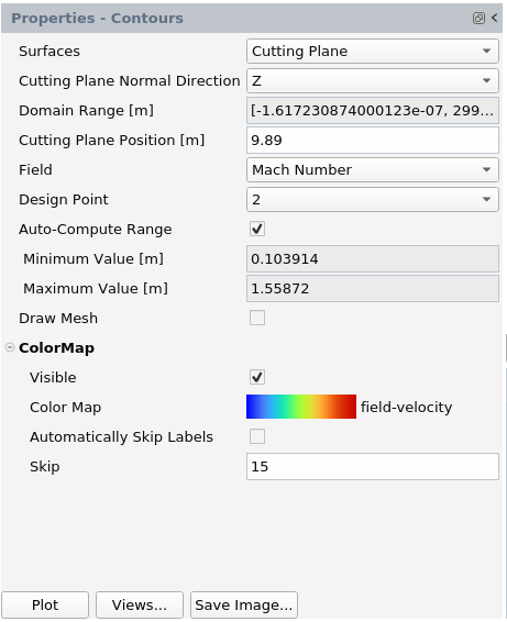
Set Surfaces to .
Set Cutting Plane Normal Direction to .
Set Cutting Plane Position [m] to
9.89which corresponds to the pylon installation position.Set Field to .
Enable .
In the ColorMap section, uncheck and set Skip to
15.Click the button to create and display the cutting plane contour in the Graphics window.
You can further adjust the contour settings from the properties panel of contour-2 from its properties panel:
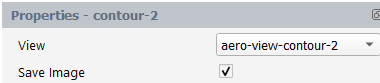
Enable the Save Image option to save the current contour image when executing the Save Current DP Images or Save All DPs Images command.
Go to the Graphics window and adjust the contour view to your preference. From the Outline View, right click on contour-2 and select Save View command. This will save the current view as aero-view-contour-2 under the View option in the properties panel.
Click Display to update the contour in the Graphics window.
The Plots options can be used to quickly display simple 2D plots of selected design points and solution variables.
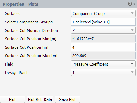
Left-click Plots. The Properties - Plots window will be displayed.
Set Surfaces to .
Change Select Component Groups to .
Set Surface Cut Normal Direction to .
Set Surface Cut Position [m] to
4which is a position close to the fuselage.Set Field to .
Click Plot and the pressure coefficient on the walls of DP-1 at Z=4m will be plotted in the Plots window.
A Plot Options panel will appear after clicking the button. You can use this panel to personalize some plot settings for both axes.
Set Axis to .
Uncheck .
Set Range/Minimum and Maximum to
25.5and37.5respectively.Set Number Format/Type to .
Set Precision to
3.Set Pattern to from Curve Settings.
Click from the Plot Options panel.
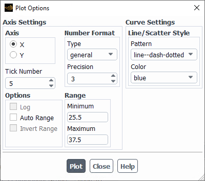
A .csv file will be saved in the Results folder after clicking the button, which is visible within the DP-1/Data folder in the Project View.
Repeat the above step for Surface Cut Position [m] of
16and28which are positions close to the mid-range and the tip of the wing respectively. After plotting the pressure-coefficient at these wing-span positions, set the Design Point to and create the same plots for DP-2. After completing these plots, the corresponding .csv files are saved to the DP-1/Data folder in the Results directory.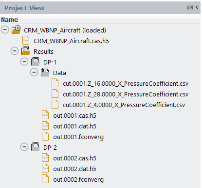
After generating all the graphics objects for design 1, you can load the solution of design point 2 and re-use these graphics objects. Select Design Point (DP-1 Loaded) and from the properties panel that appears,
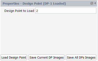
Set Design Point to Load to 2.
Click the Load Design Point button.
You can now go to the contours that you created and click Display to show these contours for design point 2.
You will now save the images of contour-1 and contour-2 for both design points.
Make sure that the Save Image flags for contour-1 and contour-2 are enabled.

Select Design Point (DP-2 Loaded) and click the Save All DPs Images button. Fluent Aero will save both contours for each design point to the Results folder.
After completing the current simulation, you can close the solver by right-clicking CRM_WBNP_Aircraft from the Outline View and selecting Close Solver. An information panel will appear to ask you if you want to save the case file or not. Click Yes to save the case file and preserve the post-processing graphics settings.
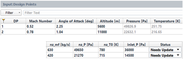
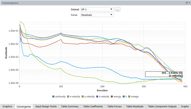
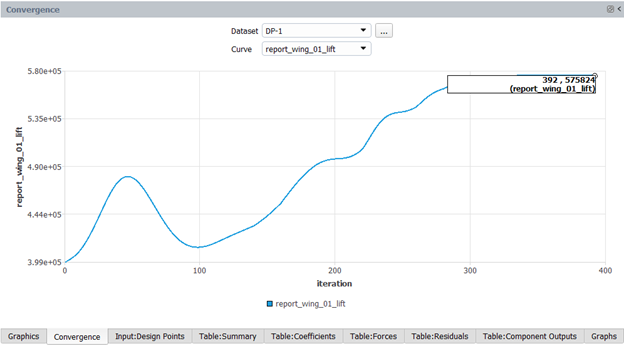
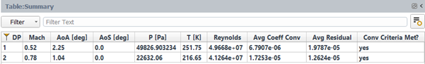
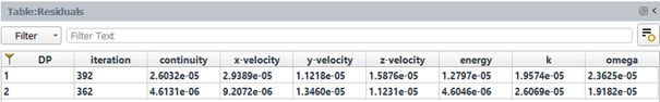
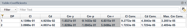
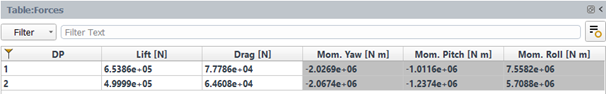
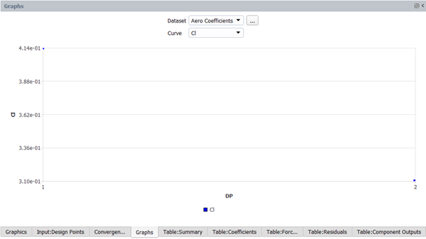
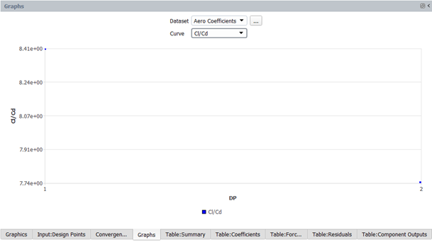
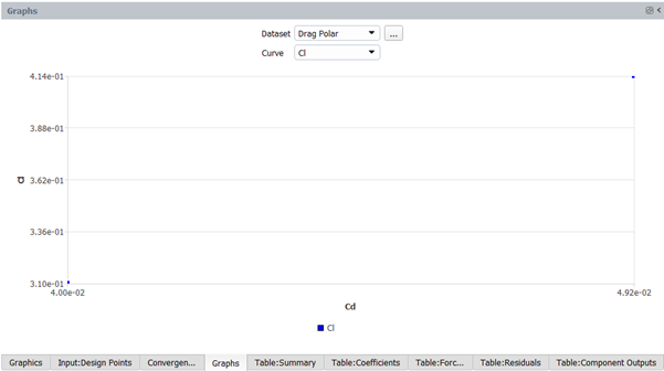
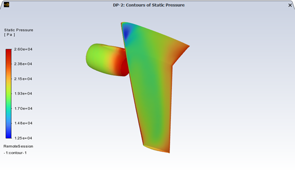
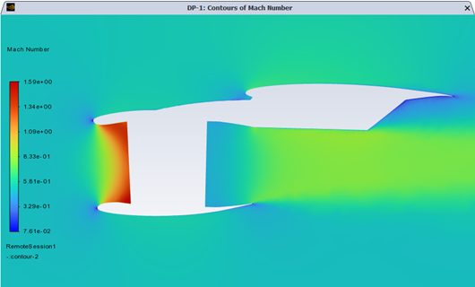
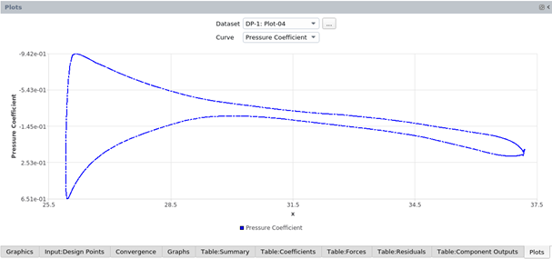
The objective of this tutorial is to introduce the workflow of the WindTunnel domain type simulation in Fluent Aero and to compute the flow around a horizontal stabilizer installed in a wind tunnel at different mass flow rates.
Download the fluent_aero_tutorial.zip file here .
Unzip fluent_aero_tutorial.zip to your working directory.
Extract the IRT-Swept-Tail-Wing.cas.h5 file and the reference_data folder for this tutorial. The reference_data folder contains several .csv formatted text files that will be compared to the results from the current calculation. These reference data files have been generated for demonstration purposes only.
The IRT-Swept-Tail-Wing.cas.h5 file contains a NACA64A008 swept tail placed inside a 1.8m high by 2.7m wide by 15.2m long test section. The chord line at the root is aligned with the center line of the wall floor of the tunnel. Thus, the airflow inside the test section is aligned with the chord of the 3D model. The objective of this simulation is to capture the wall-effects associated with the wind tunnel test section. The grid consists of 585,742 nodes, and 1,596,549 cells. This is a coarse mesh, and is used for demonstration purposes only. Tetrahedral cells define most of the computational domain. Eighteen layers of prisms are grown off the horizontal stabilizer walls. A mass-flow-inlet boundary is used to define the wind tunnel inlet flow upstream of the stabilizer. A pressure-outlet type boundary represents the wind tunnel outlet condition. The remaining four surrounding boundary zones are defined as wall and symmetry boundary types.
This mesh follows the WindTunnel domain type requirements of a Fluent Aero simulation. Refer Freestream or WindTunnel Domain Type Requirements for more information.
Launch Fluent 2024 R2 on your computer. On the Fluent Launcher panel, set the Capacity Level to . Then select Aero. Set the number of Solver Processes to
4-16. Click .Alternatively, Fluent Aero can be opened using the aero (on Linux) or aero.bat (on Windows) file inside the fluent/bin/ folder.
In the Fluent Aero workspace, go to the Project ribbon. Click Workspaces → , and check , and should remain unchecked.
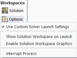
When this option is enabled, a Fluent Launcher window will open when loading a case file. This allows you to schedule a calculation on a server and/or to specify a different number of solver Processes to use in your simulation. Alternatively, if this setting is disabled, Fluent Aero will load the case file in a solver session on your local machine.
In the Project ribbon panel, select Project → and enter
Fluent_Aero_Tutorial_04to create a new project folder.In the Project ribbon, select Simulation → , and browse to and select the IRT-Swept-Tail-Wing.cas.h5 file. A New Simulation window will appear. Enter the Name of the New Simulation as
IRT-Swept-Tail-Wing, check to enable and . Click .A Fluent Launcher window will appear, set the Solver Processes to
4-16and click . The case file will open and a background solver session will load. A new simulation folder will be created in your project folder, and the IRT-Swept-Tail-Wing.cas.h5 file will be imported.After the .cas.h5 file has been successfully loaded, a new Outline View tree appears under IRT-Swept-Tails-Wing (loaded).
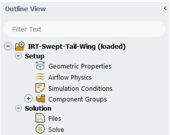
While importing, Fluent Aero will attempt to automatically determine if a WindTunnel domain type is being used. It will search for any boundary that has windtunnel in its name and add those boundaries to the WindTunnel group. If all the required boundaries are identified to create a valid windtunnel group, Fluent Aero will set the domain type as WindTunnel, and the following message will be reported in the Console.
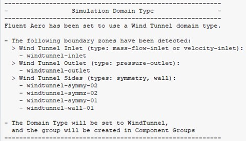
In the Outline View window, click Geometric Properties. A Properties - Geometric Properties window appears below the Outline View window. At the top of this new properties window, notice that the Domain Type has been automatically set to .
Define the orientation of the geometry within the computational domain, which will be used to compute the aerodynamic forces.
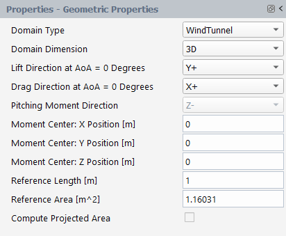
Set Domain Dimension to .
Set Lift Direction at AoA = 0 Degrees to .
Set Drag Direction at AoA = 0 Degrees to .
Pitching Moment Direction will automatically be set to .
Set the Moment Center X-, Y- and Z-Position [m] to
0,0, and0, respectively.Set the Reference Length [m] to
1, which corresponds to the mean chord length.Set the Reference Area [m^2] to
1.16031.Alternatively, the reference area can be computed by enabling the option. A pop-up panel will appear. Set the Projection Direction to and select all the surfaces of the swept wing geometry. Click the button and then click the button to copy the computed area to the Reference Area [m^2] box.
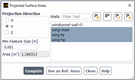
In the Setup tree, go to Airflow Physics. In the Properties – Airflow Physics window, apply the following settings:
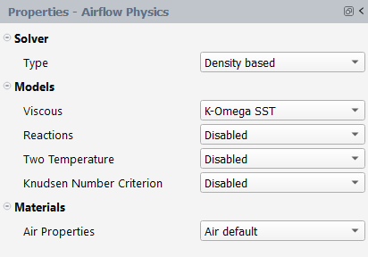
In the Solver section:
Set Type to .
In the Models section:
Set Viscous to .
Set Reactions to .
Set Two Temperature to .
Set Knudsen Number Criterion to .
In the Materials section:
Set Air Properties to .
In the Setup tree, go to Simulation Conditions.
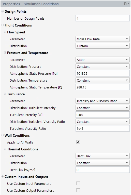
In the Properties – Simulation Conditions window:
Set the Number of Design Points to .
In the Flow Speed section:
Set Parameter to .
Set Distribution to .
Go to the Pressure and Temperature section:
Set Parameter to .
Set Distribution: Pressure to .
Set the Atmospheric Static Pressure [Pa] to
101325.Set Distribution: Temperature to .
Set the Atmospheric Static Temperature [K] to
288.15.
In the Turbulence section,
Set Parameter to .
Set both Distribution: Turbulent Intensity and Turbulent Viscosity to .
Set Turbulent Intensity [%] to
0.08.Set Turbulent Viscosity Ratio to
1e-5.
In the Wall Conditions section:
Enable .
In the Thermal Conditions section:
Set Parameter to .
Set Distribution to .
Set Heat Flux [W/m2] to
0.
An Input:Design Points table will be created in the Graphics window on the right-hand side of the user interface. This table shows all the design points that will be simulated.
Set the Mass Flow Rate [kg/s] for each DP as shown below.
The Mach Number corresponding to the Mass Flow Rate of each design point will automatically be calculated and displayed in the input design point table. The initial status of each design point (DP) has been set as .
Go to Component Groups. Two default Component Groups have been created after the simulation is loaded. The WindTunnel group contains the inlet and outlet zones that define the inflow and outflow conditions of the wind tunnel and 4 boundary zones used to represent the wind tunnel wall. The Other group contains the remainder of the boundary zones which are the walls of the wing geometry.
Create a type component group from these boundary zones.
In the Properties – Component Groups window, click . The component groups manager panel will appear.
To create a Wing type component:
Set Type to in the New Component section and a default group name Wing_01 will appear.
Change the Name to
Wing.Use to add Wing into Existing Components. All the boundary zones that have not been assigned to any group are listed in the Available Zones. A Wing type group is a specific type of group which contains a Component Parts such as Walls.
From Available Zones, select all the boundary zones that start with wing and use to add them to the Walls component parts.
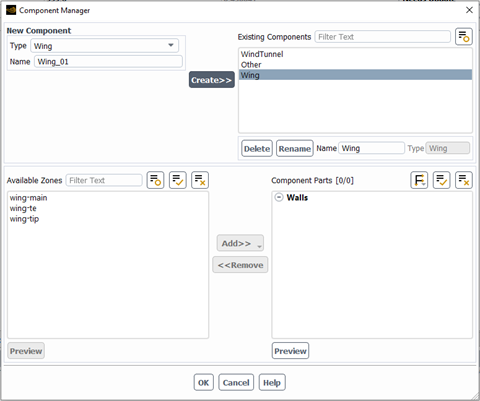
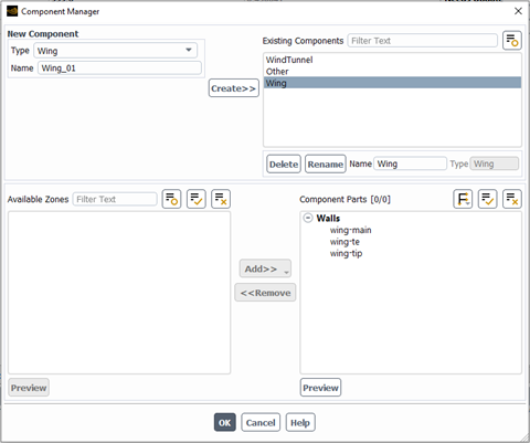
Next, enable additional output variables relevant to your components.
In the Setup tree, go to Component Groups.
In the Properties – Component Groups window:
Click the button to enable component specific output parameters.
From the Manage Component Outputs panel:
Check the box of the WindTunnel and Wing components.
Check the box of the WindTunnel component.
Because is enabled, the mass flow rate of the WindTunnel inlet and the lift and drag forces of the Wing component will be calculated and summarized in Table:Component Outputs after the calculation is complete. Since is enabled, the evolution of the mass flow rate of the WindTunnel inlet will be plotted in the Convergence plot.
Click to close this panel.
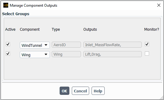
Go to Solution → Files.
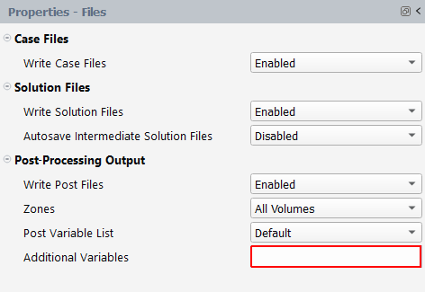
In the Post-Processing section,
Set Write Post Files to .
Go to Solution → Solve.
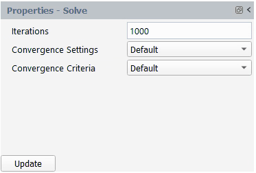
Set Iterations to
1000.Keep Convergence Settings and Convergence Criteria to .
Click the button at the bottom of the Properties - Solve panel.
The calculation will start, and the first design point, DP-1, will be simulated. A Convergence window will appear in place of the Graphics window and display the residuals and monitors for DP-1.
Design point DP-1 will continue until the total Iterations (1000) or the Residuals Convergence Cutoff (1e-5) and Aero Coeff Conv. Cutoff (2e-5) are reached, whichever comes first.
In this example, DP-1 will calculate for 1000 iterations. At that point, the conditions will be updated for the next design point and the calculation will resume. This process repeats until all design points are simulated.
Look at the convergence history of the simulation in the Convergence window located on the right of your screen. Set the Dataset to and the Curve to , to view the continuity, x-, y-, z-velocity, energy, and turbulence residuals for the first design point. You can left-click a residual curve to show the iteration number and the corresponding residual value. Here, the residual of k at iteration 1000 is shown and is roughly 3.0756e-5 which is still higher than the residual convergence cutoff (1e-5). The remaining residuals of DP-1 have met the Residuals Convergence Cutoff criteria after 1000 iterations.
Note: While only the residual of k does not meet the residual convergence cutoff criterion of 1e-5, it is still recommended for you to investigate your solutions to ensure that appropriate convergence levels have been achieved and that convergence remains stable.
In the Convergence window, set Curve to . The evolution of the drag coefficient for DP-1 will be displayed. Left-click the last iteration of the drag-coefficient plot, to show the drag coefficient value at the end of this simulation.
When the calculation of DP-1 is complete, the status column in row 1 of the Input:Design Points table will be set to , and the calculation of DP-2 will begin.
After all design points have been updated, the status of the Input:Design Points table will be set to for all the design points.
A Results node will be displayed in the Outline View tree after the simulation starts. The Results node contains a Simulation and a Design Point sub-components. This allows you to quickly post-process design point solutions, by obtaining aerodynamic coefficient plots, creating contour plots of solution fields, comparing solution fields to experimental data, and more.
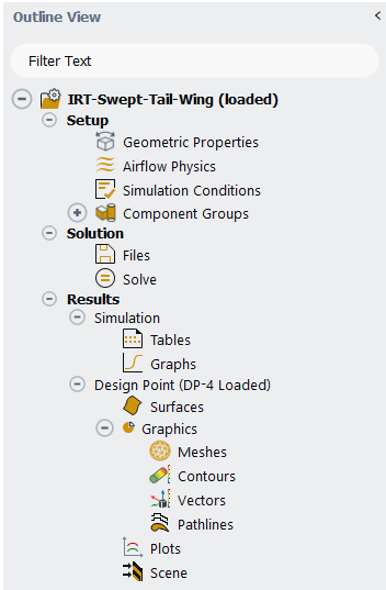
Go to the Simulation node which provides a comprehensive view of aerodynamic coefficients across all design points. The first element in the Results node is Tables. In the current tutorial, five different Tables will automatically be created in the Graphics window area when the calculation is complete.
Click the Table:Summary, Table:Coefficients, Table:Forces, Table:Component Outputs and Table:Residuals tabs at the bottom of the Graphics window to reveal each table.
Table:Summary summarizes the flight conditions and convergence information for each design point. In the current simulation, all design points have partially met the convergence criteria. However, all simulations provide stable aerodynamic coefficients that do not vary after ~500 iterations and all residuals satisfy the convergence criteria except for the k-turbulence equation. Therefore, all design point results are considered as fully converged solutions.
Table:Coefficients contains the lift and drag calculated in the wind-fixed coordinate systems, yaw moment, pitching moment and rolling moment coefficients, calculated in the body-fixed coordinate systems which are highlighted in gray. The Cl Conv. and Cd Conv. columns measure the convergence of the lift and drag coefficients, which are used to determine if the convergence criteria are met. The last column shows the maximum value of the convergence of the yaw, pitching and rolling moments.
Table:Forces contains the lift, drag and moment forces. Similar to the results in Tables: Coefficients, lift and drag forces are computed in the wind-fixed coordinate system while moment forces are calculated in the body-fixed coordinate system.
Table:Component Outputs shows the results of the selected component specific output parameters. In this tutorial, the lift and drag forces of the Wing component and the mass-flow rate of the wind tunnel inlet section are shown.
Table:Residuals shows the final residuals as well as the number of iterations run for each design point.
Click Graphs in the Outline View to show the plots of the aerodynamic coefficients and other results defined in Fluent Aero:
At the bottom of the Properties - Graphs window, click . An XY plot of lift coefficient () vs. design point (DP) will appear in the Graphics window.
Select from the drop-down list of the Curve menu to plot the drag coefficient as a function of the design point.
The moment coefficients can be shown by selecting from the Curve selection drop-down list.
Click the button. An X-Y plot will appear in the Graphics window. There is an option button located on the right of the Dataset drop-down. This button can be used to modify some of the plot settings and export the plot to the disk.
Select from the Curve drop-down menu.
Click the option button.
Select → → and change the x variable to .
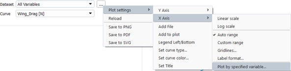
Select → (and ) → to adjust the range for the x and y axis, if required.
The plot of the drag force of the wing vs the inlet mass-flow rate of the wind tunnel will be shown.
You will now go to the Design Point (DP-# Loaded) section and visualize graphics results such as contours for a specific design point in the graphics window. After creating these graphics objects, you can easily replicate them for a different design point. From the Properties – Design Point (DP-# Loaded) panel,
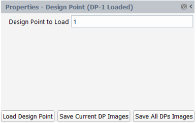
Set Design Point to Load to 1.
Click Load Design Point command to load the solution file of design point 1.
Select Contours under Graphics. There are two methods to create a contour. One way is to right-click on Contours, select New… and then specify the contour properties. Alternatively, you can predefine the properties from the Properties - Contours panel before creating the contour:
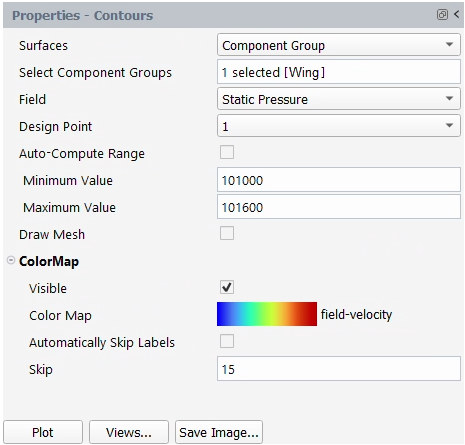
Left-click Contours from Outline View to display the Properties - Contours setup window.
Set Surfaces to .
Set the Select Component Group to .
Set the Field to .
Uncheck and set Minimum Value to
101000and Maximum Value to101600.Click to expand the ColorMap options. Uncheck and set Skip to
15.Click the button to create and display the contour in the Graphics window. A contour-1 node now appears under Contours.

In the Graphics window, use the mouse to set the view of the contour. Right-click on contour-1 and then select Save View. This will save the current view as aero-view-contour-1 under the View option in the properties panel of contour-1.

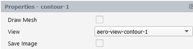
Under Properties - Contours
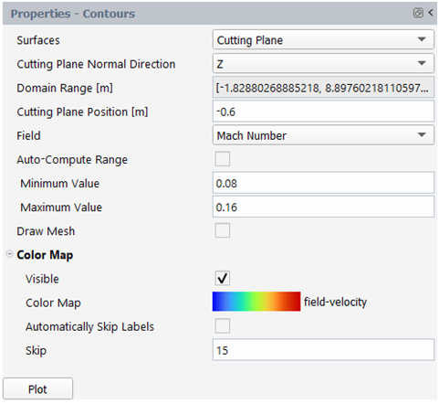
Set Surfaces to .
Set Cutting Plane Normal Direction to .
Set Cutting Plane Position [m] to
-0.6.Set Field to .
Uncheck and set Minimum Value to
0.08and Maximum Value to0.16.Uncheck and set Skip to
15.Click the button to show the cutting plane contour in the Graphics window.
The Plots options can be used to quickly display simple 2D plots of selected design points and solution variables.
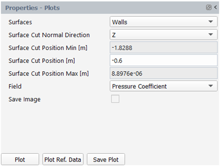
Left-click Plots. The Properties - Plots window will be displayed.
Set Surfaces to .
Set Surface Cut Normal Direction to .
Set Surface Cut Position [m] to
-0.6.Set Field to .
Click Plot and the pressure coefficient on the walls of DP-1 at Z=-0.6m will be plotted in the Plots window.
A Plot Options panel will appear after clicking the button. You can use this panel to customize plot settings for both axes. Notice that when the pressure coefficient is selected in Field, the range of the y-axis will be inverted with higher value on the bottom and lower value on the top.
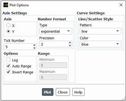
A .csv file will be saved in the Results folder after clicking the button, which is visible within the DP-1/Data folder in the Project View.
Click the button to load and plot a reference dataset in the current plot. In the dialog window that appears, browse to the reference file ref-irt-swept-wing-Cp-massflow-313-section-z0.6m.csv in the reference_data folder, and click . You can use the button to export the current plot to a .png file on disk. The reference data will be imported in the DP-1/Data folder in the Project View. The same plot settings will be applied to the Fluent Aero results and black dots will be used to plot the reference data.
In the Project View menu, a Results folder is created after the calculation starts. A folder for each design point along with an associated case file, data file, and convergence file will appear inside the Results folder. A Data folder which contains the results (a .csv formatted file) of the 2-D plot of the pressure coefficient is created.
The results can be further investigated using the Post-Analysis (Beta) tool. Right-click out.0001.dat.h5 and select . This command will load the Post-Analysis (Beta) viewer. Post-Analysis (Beta) is a Beta feature that makes use of the Post-Analysis (Beta) post-processing functionality and is directly displayed in Fluent Aero’s Graphics area. A Post-Analysis (Beta) tree node appears in the Outline View, where you can continue post-processing.
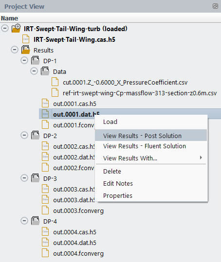
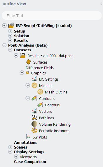
Note: The Post-Analysis (Beta) option is still a beta feature. Therefore, you may experience some limitations during use.
Two different types of solution files can be loaded into Post-Analysis (Beta) using :
, which is represented by the out.0001.dat.h5 file.
, which is represented by the out.0001.dat.post file.
When using the Post-Analysis (Beta) functionality, it is preferred to use the . The contains selected variables for post-processing and is formatted specifically for use with the Post-Analysis (Beta) tool.
Create a Contour plot using the Post-Analysis (Beta) tool:
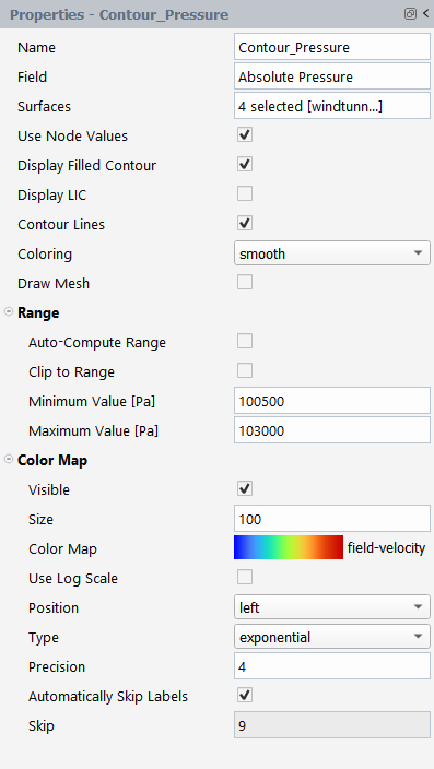
Right-click Contours in the Post-Analysis (Beta) tree and select
In the Properties panel that appears, change the Name to
Contour_Pressure.Change the Field to .
In the Surfaces selection panel, select windtunnel-wall, wing-main, wing-te, and wing-tip.
Enable .
Disable Range.
Set the Minimum Value [Pa] and Maximum Value [Pa] to
100500Pa and103000Pa, respectively.Expand the Color Map section to reveal more options.
Set the Precision of the legend to
4.Click .
The Contour_Pressure will be displayed in the Post-Analysis tab of the Graphics window.
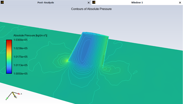
Once you are finished, you can close the dataset under Post-Analysis (Beta) by right-clicking the dataset name, Results – out.0001.dat.h5 in the Outline View and selecting .
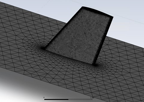
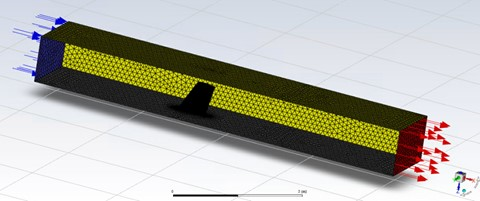
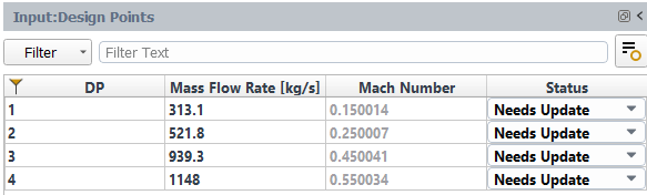
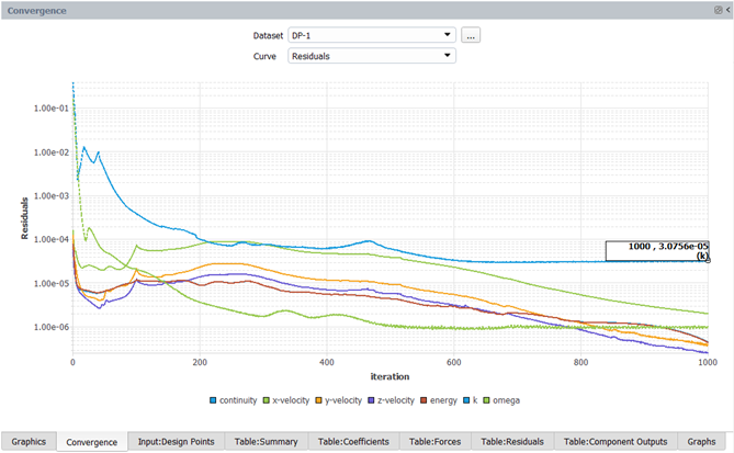
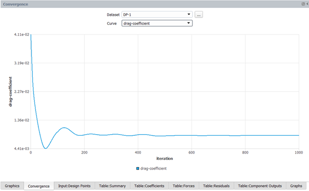
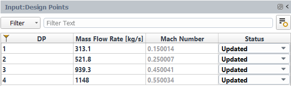
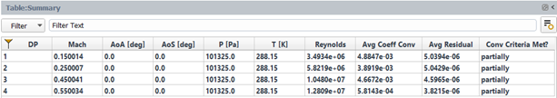
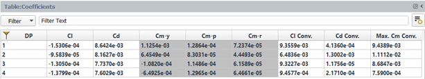
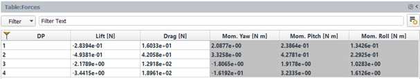
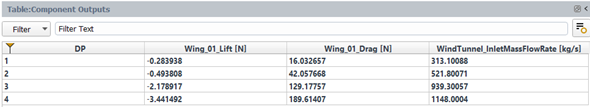
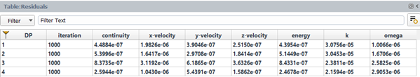
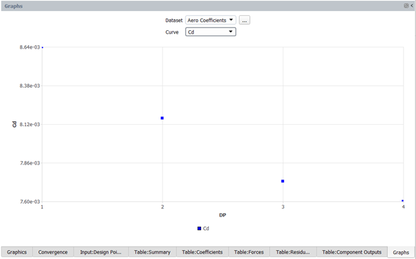
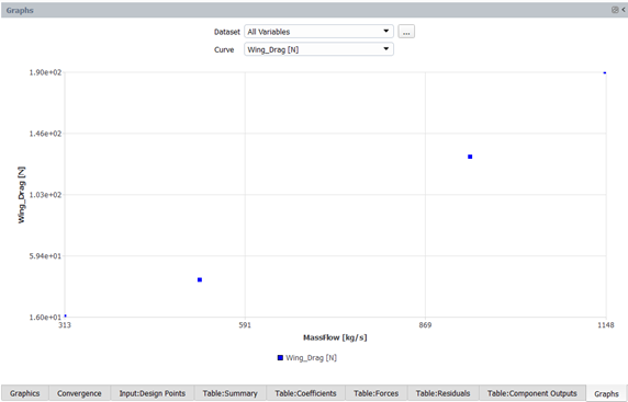
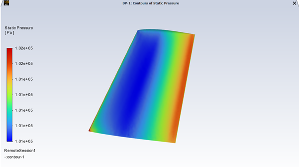
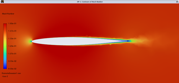
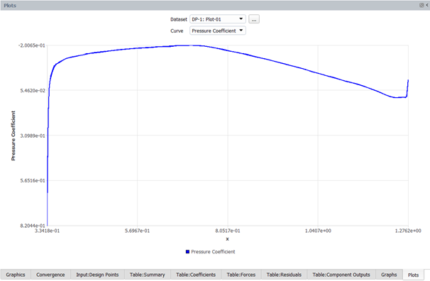
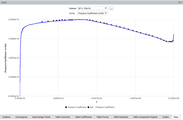
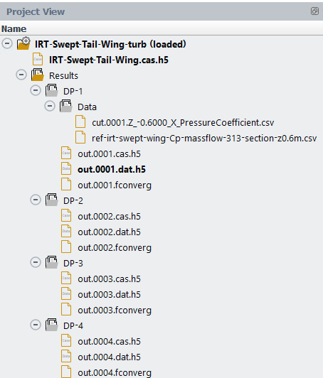
This tutorial is divided into the following sections:
The objective of this tutorial is to show how to use Fluent Aero's AET (Aerodynamic Extraction Tool) to automatically compute the aerodynamic performance of airfoil sections defined along a blade’s span. The input to the workflow is a 3D blade CAD geometry. The output of the workflow are performance lookup table files (airfoil.dat) containing lift and drag coefficients across a range of Mach, Reynolds and AoA conditions, which can be used as input to Fluent’s Virtual Blade Model in the Fluent User's Guide.
The input to this tutorial is a clean 3D blade geometry file (in SpaceClaim’s native .scdoc format) that has been prepared for use with the AET workflow. Since it has already been prepared for use in the tutorial, no special instructions are provided here. However, when using your own geometry with the AET workflow, you must prepare the geometry to meet certain requirements. Refer to AET Workflow – Preparing the Input Geometry File in the Fluent Workspaces User's Guide for more details.
Because the CAD generation step requires Ansys SpaceClaim, which is only supported on the Windows platform, the current tutorial should be completed on a Windows platform. To complete this tutorial, make sure Ansys SpaceClaim is installed (typically C:/Program Files/ANSYS Inc/v241/scdm).
Finally, this tutorial is written with the assumption that you have completed the introductory tutorials found in this manual and are familiar with the Ansys Fluent Aero Outline View and ribbon structure. Some steps in the setup and solution procedure will not be explicitly shown.
The Aerodynamic Extraction Tool (AET) is an automated workflow that extracts the performance characteristics of multiple spanwise sections of a 3D blade geometry using Ansys Fluent Aero's project and simulation capabilities, as well as the CAD capabilities of Ansys SpaceClaim and meshing capabilities of Ansys Fluent Meshing. The workflow walks you through the steps below:
Import Blade Geometry:
Select the 3D blade CAD geometry of the rotor blade that will be analyzed.
Alternatively, AET can select a 2D Points definition file of a single airfoil section to extract the performance of a single airfoil.
Extract airfoil section CADs (using SpaceClaim):
Perform multiple spanwise cuts of the 3D blade CAD to extract multiple airfoil sections using Ansys SpaceClaim as a background process.
Create Airfoil Section Meshes (Using Fluent Meshing):
Generate 2.5D meshes of each airfoil section using Ansys Fluent Meshing as a background process.
Calculate Aerodynamic Performance of Airfoil Sections:
Calculate the aerodynamic performance of each airfoil using a range of conditions using Ansys Fluent Aero’s simulations and design points.
Output Performance Lookup Table Files:
Output and save performance lookup table files containing coefficients of lift and drag computed over a wide range of Mach, Reynolds and AoA. These files will be in a format that can be used to define a rotor directly in Fluent’s Virtual Blade Model in the Fluent User's Guide.

The steps to extract the airfoil section CADs and generate the airfoil section meshes use highly automated background processes. Additional details on how each of these processes work can be found in AET: Aerodynamic Extraction Tool in the Fluent Workspaces User's Guide.
The following sections describe the setup and solution steps for this tutorial:
To prepare for running this tutorial:
Download the fluent_aero_aet_tutorial.zip file here .
Unzip fluent_aero_aet_tutorial.zip to your working directory.
The file, 3D-Blade.scdoc, can be found in the folder.
Launch Fluent 2024 R2 on your computer.
Within the Fluent Launcher, set the Capability Level to , then select Aero.
Set Solver Processes to
4-8under Parallel Processing Options.Note: You may notice slightly different convergence behavior for some design points depending on the number of CPUs used.
Click
Alternatively, Fluent Aero can be opened using the aero (on Linux) or aero.bat (on Windows) file inside the fluent/bin/ folder.
Enabling beta features will give you access to the Aerodynamic Coefficients Averaging option which will be used during this tutorial.
 File
→ Preferences... →
Aero → Beta
Features
File
→ Preferences... →
Aero → Beta
FeaturesNote: It is possible to run this tutorial with beta features disabled, and without using the Aerodynamic Coefficients Averaging feature. However, your results will not contain averaged values for design points that feature oscillating solutions. Therefore, the workflow and results may be slightly different than those shown in this tutorial.
Create a new project file.
File → New
Project...
Enter
Fluent_Aero_Tutorial_AETas the Project file name within the Select File dialog.Create a new AET workflow.
File → AET
Workflow → New... Select Input CAD Mode → from the New AET Workflow dialog box.
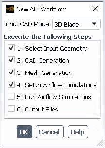
Keep all other default settings. This default configuration instructs the AET workflow to automatically proceed to the airflow simulation setup step, where the airflow simulations for each airfoil will be created and ready to launch. Click to close the window.
Note: If you are already familiar with the AET workflow, you can enable all steps. The AET workflow will then automatically work through all its steps and output the final VBM required lift/drag tables in *.dat file format.
The step uses SpaceClaim which is only supported on the Windows platform. Therefore, this step must be done on Windows. All other steps are supported on both Linux or Windows platform.
If you would like to perform the remaining steps on the Linux platform (for example, to access additional CPUs to calculate your airflow simulations more efficiently), you could break down the AET steps as follows:
Execute to on Windows.
Zip your entire project folder and project file (projectname.flprj, projectname.cffdb).
Transfer the zip folder to Linux.
Unzip and use
File
→ AET
Workflow → Continue...
to restart from and continue on to later
steps.
Navigate to select the input CAD file, 3D-Blade.scdoc, from the Select File dialog box.
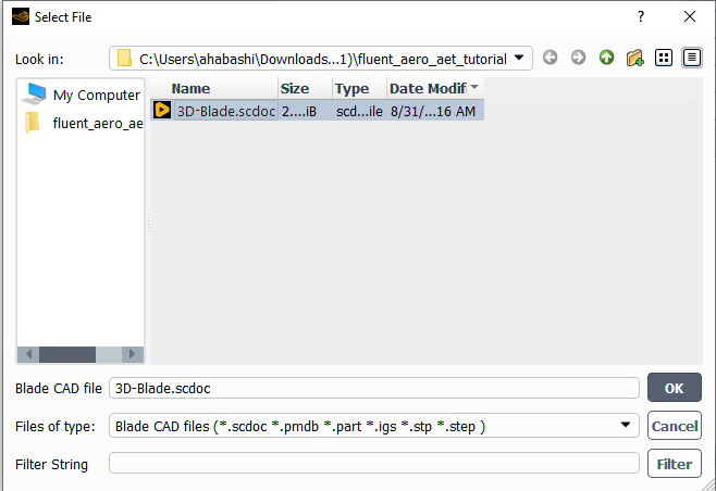
Define section locations along the 3D blade through the Define Blade Sections dialog box.
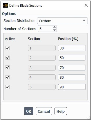
In the Options section,
Set Section Distribution to .
Set Number of Sections to .
Set Position [%] to
30,50,70,80, and90, respectively.
Note: When setting up the section positions, it’s important to ensure that the minimum and maximum position percentages are defined such that they intersect a blade section of the geometry. The 0% position corresponds to the center of rotation and 100% position corresponds to the blade tip position. In this case, 30% is used as the minimum position and corresponds to an airfoil section nearest to the root of the blade.
Set up airflow simulations through the Define Airflow Simulation Settings dialog box.
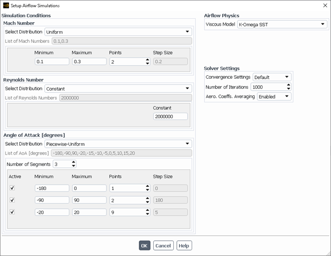
In the Options section,
Set Section Distribution to .
Set Number of Sections to .
Set Position [%] to
30,50,70,80, and90, respectively.
Click to close the window.
Note: The Select Distribution of Airflow Conditions section defines the design points that will be simulated. All combinations of Mach Number and Angle of Attack [degrees] will be represented in the table due to the use of and distributions, resulting in 24 design points for each airfoil profile. All of these points were chosen with the goal of providing a complete and sufficient set of aerodynamic performance data for Fluent's Virtual Blade Mode (VBM). Some thoughts on the selection of these design elements.
Two Mach Numbers (0.1 and 0.3) are used to evaluate the aerodynamic performance of the blade section under different flow ranges that the airfoil could encounter. More Mach numbers could be used to evaluate additional flow ranges.
A total of 12 design points will be used to simulate the angles of attack (between -20 and 20 degrees) that will most frequently be experienced by the blade section. In the current demonstration, this results in a step size of 5 degrees between consecutive angles of attack. This is a relatively high step size and is used in this tutorial to reduce its computational cos. For increased precision, this section could be further refined or expanded to evaluate more points. For example, you could consider evaluating a step size of 1-2 degrees or a range of angles between -30 and 30 to offer a more complete set of design points.
Three design points will be used to simulate very large angles of attacks, notably at 180, 90 and -90 degrees. These angles will create the set of design points allowing Fluent’s VBM to have a complete set of data that can be used to interpolate all possible angles of attack of the blade section. It is required to provide Fluent’s VBM with data that covers the entire range of angles of attack as it is essential to simulate at least the 180 degrees angle of attack.
The AET workflow will begin:
Extracting a section profile from the input 3D blade geometry.
Generating a 2.5D mesh for each airfoil profile.
Setting up the airflow simulations.
When complete, you’ll see the output files listed in the Project View.
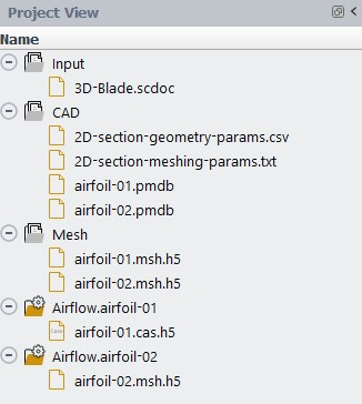
Despite the fact that you are extracting five airfoil sections from the 3D blade geometry (30%, 50%, 70%, 80%, and 90% span), only two CAD and mesh files have been generated (airfoil-01.cas.h5, airfoil-02.cas.h5, and airfoil-01.msh.h5, airfoil-02.msh.h5). This occurs after Fluent Aero determined that some of the sections share the same underlying airfoil shape (they may simply differ in chord length or twist), and therefore, the performance calculations are only required for one of the shared sections. The 50%, 70%, 80%, and 90% spanwise blade sections all have the same shape in this case. More information about the blade sections can be found in the CAD folder's 2D-section-geometry-params.csv file.
Note:You can review the different outputs of the AET workflow CAD generation step from the …/CAD/ directory.
sc-script.log
Contains detail printouts of SpaceClaim generating the 2.5D CADs. You can refer to this file for more information should there be any failure in the CAD generation step.
sc-script.png
Contains a figure which shows the sections defined along the input 3D blade geometry.
sc-script.scdoc
CAD file containing all related geometries during the generation of 2.5D CADs.
2D-section-meshing-params.txt
Input file to the AET workflow Fluent Meshing step.
2D-section-geometry-params.csv
Contains summaries of the 3D blade geometry and 2.5D sections. This file contains information helpful in setting up the definition of the blade in Fluent’s VBM model.
airfoil-*.pmdb
SpaceClaim outputs of 2.5D CADs extracted airfoil profiles used as inputs in the Fluent Meshing step.
You can also review the outputs of the AET workflow mesh generation step from the …/Mesh/ directory.
airfoil-*.msh.h5
Fluent Meshing 2.5D mesh used for the airflow simulation in later steps.
airfoil-*-fluentMeshing.log
Fluent Meshing log file for a specific airfoil profile generated by the 2.5D mesh. You can refer to this file for more information should there be any failure in the mesh generation step.
airfoil-*-2D-remeshing.jou
Script executed by Fluent Meshing to generate the 2.5D mesh for a specific airfoil profile.
airfoil-*-2D-meshingSizes.scm
Contains mesh settings for a specific airfoil profile.
The following files are templates that define the meshing parameters and boundary geometry provided by the AET workflow:
2D-meshingSizes.scm
2D-remeshing.jou
create-2.5D-mesh.bin
FARFIELD-SYMMS.msh.h5
DENSITY-BOX-01.pmdb
DENSITY-BOX-02.pmdb
DENSITY-BOX-03.pmdb
Before launching airflow calculations, you can load simulations for a specific airfoil to review its list of design points and settings and make any necessary changes.
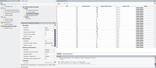
For example, with
Project
View → Airflow.airfloil-02
selected, go to Project
→ Simulation → Load
Simulation.The design point table and airflow settings will be visible within Fluent Aero's graphical user interface.
Close the Airflow.airfloil-02 simulation once your changes are applied. Click to save the case file when closing the simulation.
Project
→ Simulation → Close
SimulationAfter making a change to an individual airflow simulation, you can copy the updated settings to all other airflow simulations by right-clicking the newly modified simulation.
Project
View → Airflow.airfloil-0*
[Optional] If you want to run your airflow calculations on another machine (for example, a computer cluster), copy your project files to the cluster machine and follow the steps below. Skip this step if you want to continue with the airflow calculations on the same machine you used for steps 1-9.
Close both your project and Fluent Aero on your local machine.
Copy the project file, folder and contents (Fluent_Aero_Tutorial_AET.cffdb and Fluent_Aero_Tutorial_AET.flprj) to your cluster machine.
On your cluster machine, launch Fluent Aero, and import your project using
File
→ Open Project... and selecting
the Fluent_Aero_Tutorial_AET.flprj
file.Continue with the remaining steps in this tutorial.
Continue the AET workflow to perform airflow simulations and export the VBM .dat files.
File → AET
Workflow → and
selecting the Fluent_Aero_Tutorial_AET.flprjUnder Restart from Step, select from the Continue AET Workflow dialog box. Enable to automatically export the VBM .dat files at the end of the airflow calculations.
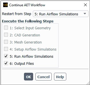
Note: If necessary, you can use the Continue AET Workflow dialog box to restart from any previous step.
Click to launch the airflow simulations of all extracted airfoil profiles.
The AET workflow will start the airflow calculations and simulate the first design point, DP-1 under Airflow.airfoil-01. The residuals and monitors for DP-1 will be displayed in the Convergence window.
DP-1 will run until the default convergence criteria for all residuals (1e-5) and lift and drag monitors (1e-4) are met, or until the maximum number of Iterations (1000) is reached, whichever comes first.
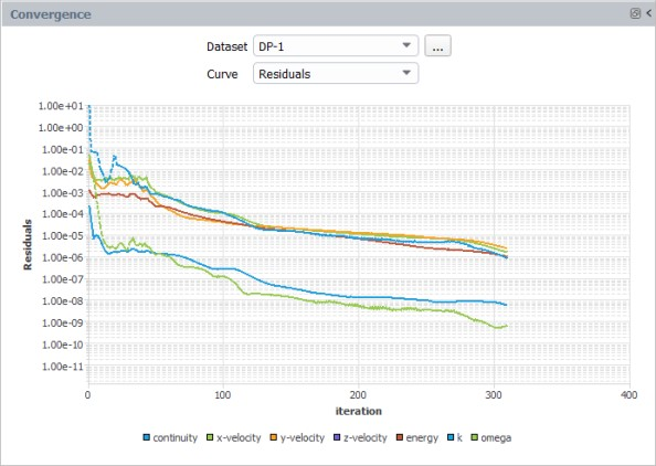
The calculation of simulation Airflow.airfoil-01 will continue until all design points have been calculated. After each design point has been updated, the Status column of the Input:Design Points table will be set to .
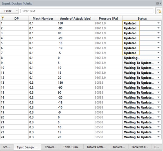
When all of Airflow.airfoil-01's design points have been calculated successfully, the simulation will close and Airflow.airfoil-02 will be loaded and its design points calculated. This procedure will be repeated until all design points of all airfoil simulations have been completed. It can take a few hours to complete this process.
Note: When you use
File
→ AET
Workflow → to
continue the airflow simulations, only design points that are not
set to are calculated. If all design
points in a single airfoil simulation are updated, the airfoil
simulation is skipped entirely. If you want to force a rerun of the
updated design points, open the airfoil simulation manually and set
the Status of all design points to
with the command below. Solution → Solve Next, select to save this status to the project.
Solution → Solve The design points will be recalculated the next time you continue the AET workflow.
The AET workflow will export the aerodynamic coefficients to airfoil-*.dat files in the output directory once all design point calculations for all airfoil simulations are completed. These files are in a format that Fluent's Virtual Blade Model can read.
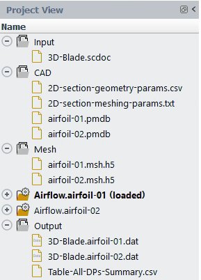
However, you should review all calculations at this point to ensure that all design points have properly converged. You can validate these results by using the tables that summarize the convergence of all design points in all airfoil simulations, or by opening individual airfoil simulations to investigate further.
Note: Some Fluent Aero airflow solver settings have been used as default settings in AET workflow airflow simulations and are suitable for most cases, with the exception of specific airfoil geometries and airflow conditions, particularly in simulations for high degree angle of attack sweeps or angles near stall. Large airflow separation and transient flow may not converge within the computational domain. Before using the design point output tables, always check the convergence of your design points and make any necessary adjustments or recalculations. This procedure is further explained in the sections that follow.
After the output step is completed, three tabs appear in the Graphics area. Convergence, Table:All DPs Summary, and Table:All Simulations Summary.

The Convergence tab displays the convergence of any design point for all airfoil simulations.
The Table:All DPs Summary tab summarizes the input parameters and convergence residuals of all design points for all airfoil simulations and is similar to Table: Summary available when an individual airfoil simulation is loaded.
The Table:All Simulations Summary tab displays design points related to all simulations which have met the convergence criteria.
Click Table:All Simulations Summary to display its contents. Notice that for airfoil 1, 16 of the 24 design points met the convergence criteria (that is, the solver residuals and aerodynamic coefficients converged below the default cutoff condition), 1 partially met the convergence criteria, and 7 did not. Design points that did not meet or met only partially the convergence criteria should be investigated.
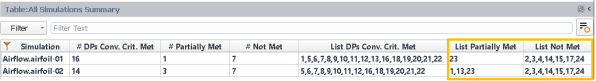
As shown in Table:All DPs Summary, these design points correspond to angles of attack of -90, 90, and -20 degrees for the Mach 0.1 condition and angles of attack of -90, 90, 15, 15, and 20 degrees for the Mach 0.3 condition. Large angles of attack are more likely to have large separation zones and difficulty converging, or have solutions with unsteady flow, such as oscillating behavior. If a design point exhibits unsteady flow-like oscillating behavior, the performance characteristics of that design point can be summarized using Aerodynamic Coefficients Averaging, see Fluent Aero - Aerodynamic Coefficients Averaging in the Fluent Beta Features Manual for more details. If not, the design point must be recalculated with more robust solver settings. This procedure is detailed in the following steps.
Select Airflow.airfoil-01 under the Project View and open its airfoil-01 simulation file.
Project
→ Simulation → Load
SimulationAll airfoil-01 related simulations will be loaded. To examine the convergence result of each design point, go to the Conv Criteria Met? column in Table:Summary and the Avg. Coeffs? column in Table:Coefficients.
Follow the guidelines below to examine the convergence of each design point.
Examine if a design point reaches convergence criteria under the Conv Criteria Met? column within Table:Summary.
If Conv Criteria Met? is , the airflow solution reached a steady state and the calculation met the converge criteria. For example, DP-1’s and are shown below. Since this design points has sufficiently converged, further calculations are not required.
If Conv Criteria Met? is or , the airflow solution did not reach a steady state and the converge criteria is not met for all or part of the criteria. The airflow can be diverged or oscillating within the domain. In this case, it is recommended to further investigate the design point.
Next, examine if the airflow solution is oscillating and if coefficient averaging has been applied. Go to the Avg. Coeffs? column within Table:Coefficients. This column is displayed when the Aero Coefficient Averaging model is enabled, which is the default setting of the AET workflow. The Aero Coefficients Averaging model will be applied and average the post processed aero coefficients if the airflow solution is oscillating in a stable pattern for more than four periods. See Fluent Aero - Aerodynamic Coefficients Averaging in the Fluent Beta Features Manual for more details. By using this model, you can extract the average value of the lift and drag coefficients when a solution features oscillating unsteady behavior in the steady state solution which may be common for design points featuring high angles of attack. While these averaged lift and drag values may not necessarily be the same as the averages of full unsteady flow calculations, they may be sufficient for use in the performance look-up tables of Fluent’s VBM model. By using this model, you will not need to rerun the design point to achieve a steady state solution, which may be unattainable for some very high angles of attack.
If Avg. Coeffs? is , the airflow solution is oscillating and the average model is applied successfully. The aero coefficient is averaged and displayed. For example, DP-2 indicates that it has not met its convergence criteria. However, Aero Coefficient Averaging has been applied. Its and curves are shown below. Notice that the lift coefficient is oscillating in a repeated way for more than 4 periods. Therefore, the average lift coefficient (Cl) is presented as the value of -9.944e-02 inside the table. Because the averaging was successful, you can keep the results of this design point and proceed to investigate the other DPs.
If Avg. Coeffs? is , the Aero Coefficient Averaging model was not applied. In this case, you need to investigate this design point further. For example, DP-15 indicates that its has not met its convergence criteria and the averaging model is not able to average the aero coefficient. Its and curves are shown as below.
This design point must be rerun with Convergence Settings set to . Go to Input:Design Points and set DP-15’s Status from to .

Set your Solve settings.
Solution → Solve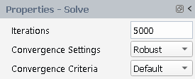
Set Iterations to
5000.Set Convergence Settings to .
Set Convergence Criteria to .
Click to re-calculate DP-15’s airflow.
Wait for the simulation to be completed. DP-15’s status will automatically be updated. The updated Residuals and lift-coefficient curves are shown below.
From the lift -coefficient monitor, a stable oscillation has been achieved, the Avg. Coeffs? of DP-15 is now set to and the averaged lift-coefficient (Cl) is presented as -2.1489e-03 inside Table:Coefficients.
Repeat the guideline above to examine each design point of Airflow.airfoil-01 to ensure the convergence criteria has been met or the aerodynamic coefficients averaging features has been applied for all design points.
In this tutorial, only DP-15 from Airflow.airfoil-01, and DP-17 from Airflow.airfoil-02 were required to be recalculated using more robust convergence settings.
Note: For more efficient recalculation of many design points, it is possible recalculate a group of design points from multiple sections sequentially (For example, DP-15 from Airflow.airfoil-01, and DP-17 from Airflow.airfoil-02) by following the steps below.
Load to the first airflow simulation.
Project
View → Airflow.airfoil-01 .In the Input:Design Points table, change the Status of any design points you would like to recalculate to , in this case, DP-15.
Set your Solve settings.
Solution → SolveSet Iterations to
5000.Set Convergence Settings to .
Set Convergence Criteria to .
Set your Simulation Conditions
Setup → Simulation
Conditions .Close the simulation and save the case.
Project
→ Close SimulationIn the Information dialog box, press to save the case.
Load the next airflow simulations and repeat steps 1 through 5 for any other design points you would like to recalculate, in this case, Airflow.airfoil-02 and DP-17.
Once the above steps have been completed for all design points you would like to recalculate, select
File → AET
Workflow → Continue...In the Continue AET Workflow dialog box, set Restart from Step to . Fluent Aero will sequentially connect to each airfoil simulation and recalculate any of the design points set to .
If you are still having difficulty with convergence for a specific design point, you have a few options to consider in order to finish your project.
To begin, change Convergence Settings to and experiment with different custom solver settings to try and improve the convergence of the design point. Use the CFL approach, for example, with a range of
10to50to allow the airflow solver to converge.Second, if you are unable to converge the design point, you can delete it from the airfoil simulation and essentially remove that angle of attack point from the final aerodynamic performance look-up table file. All design points may not be required to generate a sufficient dataset for all airfoil sections.
Next, create a Parametric Graph to further post-process the design point results.
Results → Graphs → Parametric
GraphIn the Curve Settings section,
Set Color to .
Keep all other default settings.
Click . The curves of lift vs. AoA will be plotted as shown.
The results for Mach 0.1 and Mach 0.3 calculations are similar, with the exception that the stalling angle of attack appears to be lower for Mach 0.3 than for Mach 0.1. A larger difference between the curves would most likely be seen if a higher Mach number was used. This, however, was not required for the current tutorial.
Repeat Step 14 to examine the results of Airflow.airfoil-02’s simulations. The lift curve of Airflow.airfoil-02 will be plotted as shown.
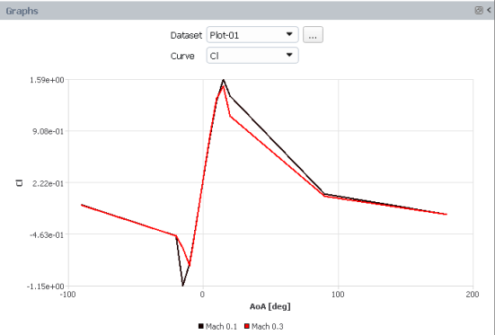
Now that a new solution has been obtained for Airfoil-01's DP-15, the output files should be updated. Use
File
→ AET
Workflow → Continue... to
restart from the step.The AET workflow will update its output files automatically. After that, go to the AET project directory ../Output/ and open airfoil-*.dat. The final AET output files for the Airflow.airfoil-01 profile are shown below.
If design points from multiple airfoil simulations are required to be rerun with settings, it may be easier to update them all together instead of calculating each individual airfoil simulation manually as shown above.
First, set and save the status of all design points required to be rerun with settings from each airfoil section to . For example, if DP-15 from each airfoil needs to be updated:
Load to the first airflow simulation.
Project
View → Airflow.airfoil-01 .In the Input:Design Points table, change the Status of any design points you would like to recalculate to , in this case, DP-15.
Set your Simulation Conditions
Setup → Simulation
Conditions .Close the simulation and save the case.
Project
→ Close SimulationIn the Information dialog box, press to save the case.
Load Airflow.airfoil-02 and repeat steps 1 through 5.
Once the above steps have been completed for all design points you would like to recalculate, select
File
→ AET
Workflow → Continue...In the Continue AET Workflow dialog box, set Restart from Step to and ensure is also selected under Execute the Following Steps. Click OK.
When is executed, Fluent Aero will identify that Airflow.airfoil-01 and Airflow.airfoil-02 have a single design point that and will sequentially connect to each airfoil simulation and recalculate that particular design point (DP-15). Since no other design points require update (the Status of all other design points is ), no other design points will be recalculated.
When is executed, the output files will be recreated and the Summary and Convergence tables will appear. Investigate these tables to ensure Airlfow.airfoil-01:DP-15 and Airlfow.airfoil-02:DP-15 have now converged.
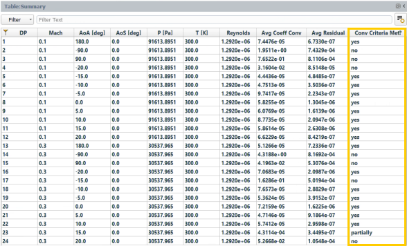
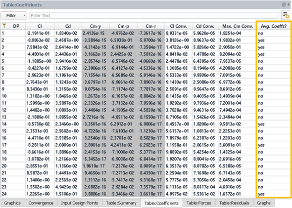
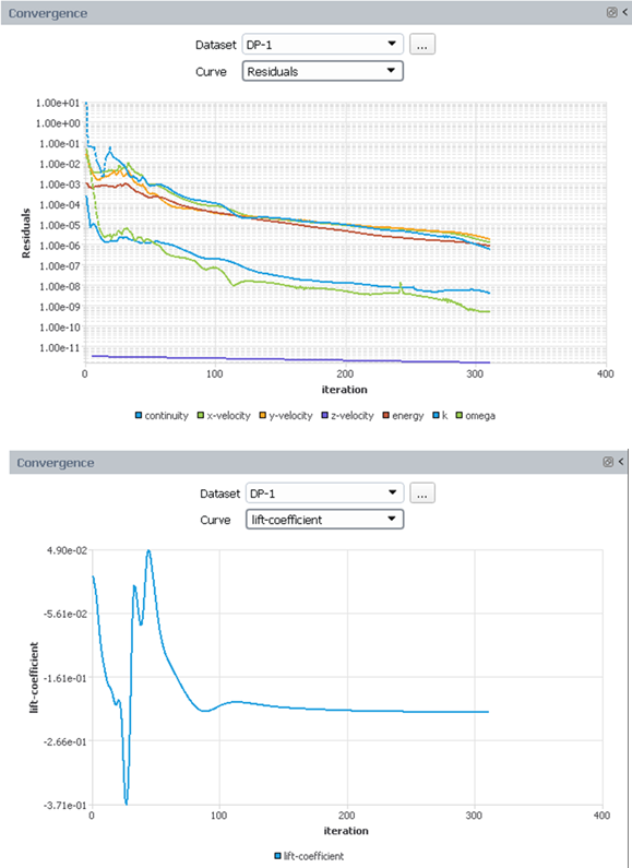
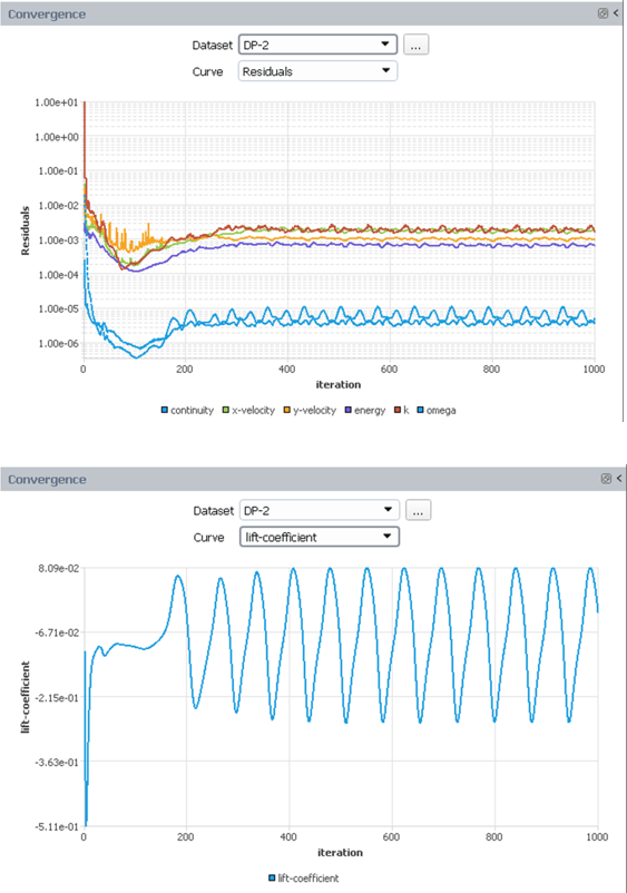
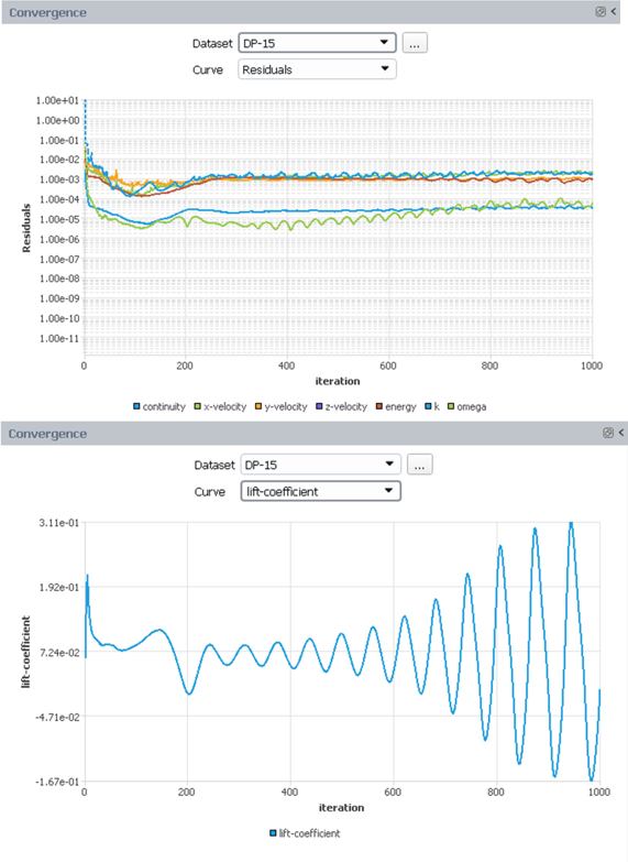
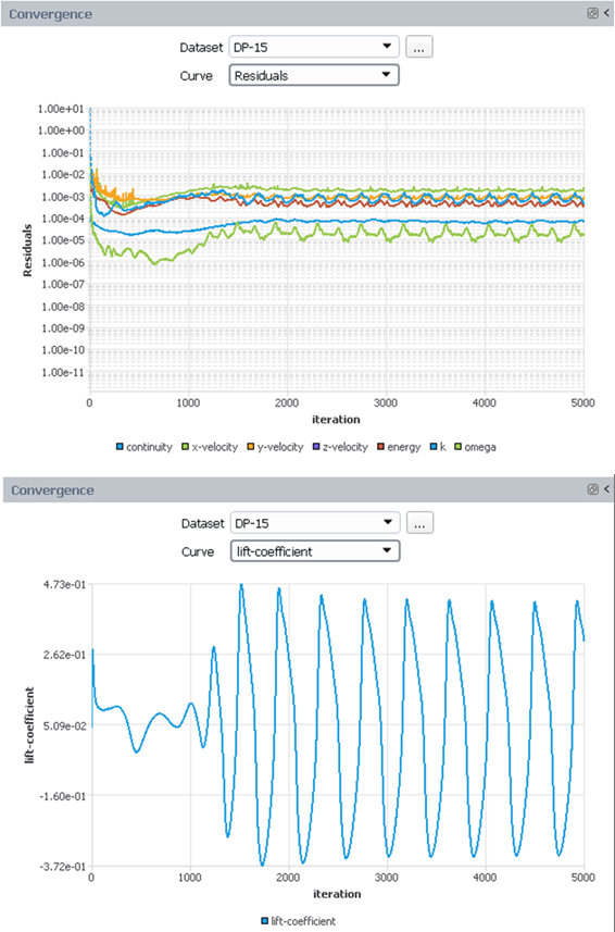
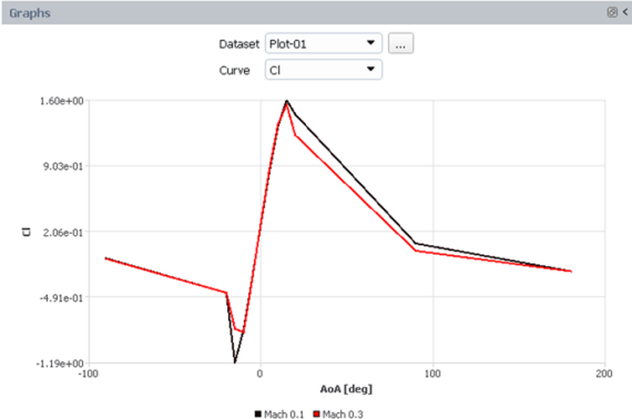
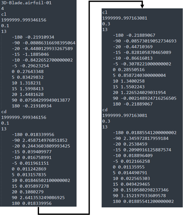
The following sections describe how to visualize your results within the Fluent Virtual Blade Model:
After completing the AET workflow, the next step is to run a Fluent simulation with the Virtual Blade Model. If you only want to simulate a single flight condition, you can do so in the classic Fluent Solution workspace. Fluent’s Virtual Blade Model Tutorials in the Fluent Tutorials contain instructions on how to run a VBM simulation using the Fluent Solution workspace. In this setup process, the following files produced by the current AET workflow tutorial can be used:
Output/3D-Blade.airfoil-0*.dat
These files define the performance of each airfoil and should be used in the Geometry panel under the VBM Rotor Inputs dialog box.
CAD/2D-section-geometry-params.csv
This file contains geometric information about each section’s position and orientation along the 3D blade. Information in this file could be helpful in setting up the Geometry panel under the VBM Rotor Inputs dialog box.
You have two airfoil performance files based on the results of the current tutorial:
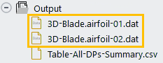
And the contents of 2D-section-geometry-params.csv are as follows:
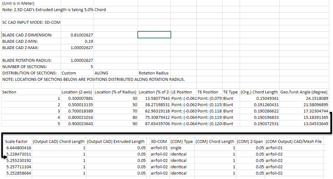
These inputs can be used in the Geometry panel under the VBM Rotor Inputs dialog box, as shown below:
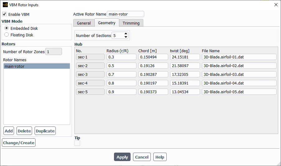
Fluent Aero can be used to utilize the Virtual Blade Model with a parametric sweep of design points. However, because the Virtual Blade Model is not yet directly available in Fluent Aero and, therefore, would need to open a Fluent Solution workspace via the Fluent Aero graphical user interface to start the setup process.
![]() Project →
Workspaces → Solution
Project →
Workspaces → Solution
This should be considered beta functionality and a basic guide to this process is provided below.
Create a new project file.
File → New
Project... Enter
VBM_helicopter_tutorialas the Project file name within the Select File dialog.Select and import the VBM_helicopter_tutorial-setup.cas.h5 input grid found inside your fluent_aero_aet_tutorial.zip folder.
Note: This file was produced by following the steps in Fluent’s Virtual Blade Model Helicopter Tutorial in the Fluent Tutorials, with minor changes to the boundary names to ensure the WindTunnel Component Group is setup automatically by Fluent Aero (the inlet, exit and wall boundaries are renamed to windtunnel-inlet, windtunnel-outlet and windtunnel-wall, respectively, and the Named Expressions are updated to match the new boundary names).
Project
→ Simulation → New Aero
Workflow A New Simulation window will appear. Enter the Name of the New Simulation as
VBM_helicopter_tutorial_custominput.Your Project View will now contain an input folder and file.
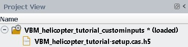
Define the Airflow Physics of the simulation.
Setup → Airflow
Physics.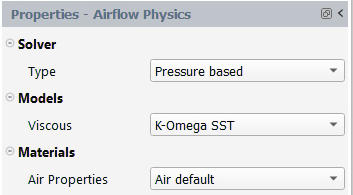
In the Solver section:
Set Type to . (Currently, Fluent’s Virtual Blade Model only supports the solver.)
Keep all other default settings.
Set your solver settings.
Solution → Solve .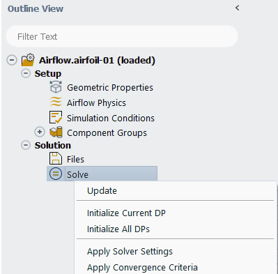
This will apply the solver condition and any other conditions that were set up in the Fluent Aero workspace and the Fluent Solution workspace.
Copy all airfoil performance lookup table files, such as 3D-Blade.airfoil-0*.dat, to the simulation folder. They will now be located inside the same directory as your primary case file, for example, VBM_helicopter_tutorial-setup.cas.h5.
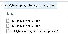
Launch the Fluent Solution workspace.
Project
→ Workspaces → Solution 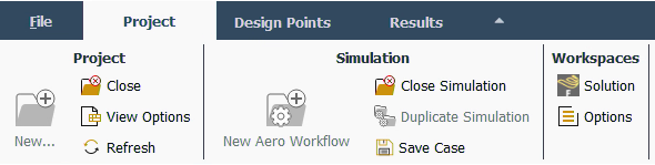
Enable the Virtual Blade Model from the Fluent Solution workspace window.
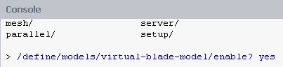
In the Console, type the following:
/define/models/virtual-blade-model/enable?
                                            yes
Initialize the airflow calculation using standard initialization. This allows VBM access to the surfaces objects for use in defining the rotor surfaces.
In the Console, type the following:
/solve/initialize/initialize-flow
Set up all required VBM Rotor Inputs to define your rotor inputs.
Setup → Models → Virtual
Blade Model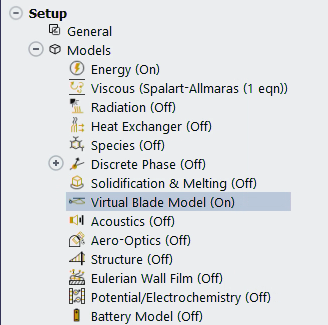
Refer to Fluent’s Virtual Blade Model Tutorials in the Fluent Tutorials for more information on this step. After finishing your setup, click to save the changes. Press to close the panel.
Apply the Virtual Blade Model.
In the Console, type the following:
/define/models/virtual-blade-model/apply
Run your calculation in the Fluent Aero workspace
Solution → Solve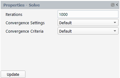
Set Iterations to
1000.Set Convergence Settings to .
Set Convergence Criteria to .
Click .
The Virtual Blade Model conditions that were set up in the Fluent Solution workspace will be used for all design points.
This tutorial demonstrated how to use Fluent Aero's AET workflow to extract the aerodynamic performance from sections defined along a 3D blade geometry and to export that data to a performance lookup table file suitable for use with Fluent’s Virtual Blade Model.