SBR+ Range-Doppler Solution Setup

The Range-Doppler Setup Type option within the SBR+ Solution Type provides a highly optimized simulation capability for range-Doppler radars, such as are commonly found in modern automotive radar sensors and also many aerospace applications. It simulates what a range-Doppler radar will observe looking into a complex environment, such as a traffic scenario or, for an airborne radar, objects on the ground. The results are presented as range-Doppler color-map images. The SBR+ radar simulation is massively accelerated relative to conventional implementations using Ansys's proprietary Accelerated Doppler Processing (ADP) technology. ADP also provides improved image quality by eliminating Doppler artifacts of the ray-tracing solution.

Range-Doppler radars operate by issuing a sequence of many pulses or chirps across a coherent processing interval (CPI). The received signal from each chirp is used to develop a time response, which is then scaled as range (distance) under the assumption of a monostatic radar configuration (that is, one where the radar Tx and Rx antennas are nearly in the same location). The range response is discretized into range bins (pixels).Then, by comparing and Fourier processing the phase response across the multiple chirps comprising the CPI, the radar develops a Doppler velocity response for each range bin. The result is a 2D range-Doppler image. Two radar waveforms are supported: pulse-Doppler and chirp-sequence frequency-modulated continuous wave (CS-FMCW).

With the Range-Doppler Setup Type, both the radar antennas and scene objects in the surrounding environment are assigned motions (for example, linear velocities, accelerations, rotations) in the History tree that depend on a user-defined time variable. Through the main dialog of this setup type, radar processing specifications are configured in terms of center frequency and range-Doppler performance specifications: range and velocity resolutions and periodic (aliasing) ambiguities. Simulation can either be performed at a single time step or, via Optimetrics, a sequence of time steps. ADP massively accelerates the simulation by eliminating the need to separately solve the hundreds of individual chirps across the radar’s CPI in microscopic time-stepping of the dynamic scene. This acceleration technique carries the side benefit of eliminating Doppler simulation artifacts caused by abrupt changes in some ray paths between chirps of the CPI.

The Range-Doppler Setup Type has a special Range-Doppler report type for displaying the range-Doppler images in color scale. These can animated according to the Optimetrics time sweep, either in a separate window or together with the 3D scene.

Prerequisites

Requirements and restrictions for Range Doppler Setup Type in SBR+ Solution Type:

• A user-defined time variable that governs the motion of objects through expressions in coordinate system definitions or Modeler tree motion operations.
• Two or more radar antenna ports defined as either built-in parametric antenna with Far-Field Source, imported far-field antennas, or far-field links to a source design. Near-field links are not supported with the Range-Doppler Setup Type.
• The range-Doppler setup is not compatible with Incident Plane Wave excitation and RCS simulations.
• Moving objects that interact with the radar must be imported as 3D Components.
• Stationary objects may defined within the range-Doppler design in the usual fashion.
• Material treatments applied to all scattering objects in the usual fashion of the SBR+ Solution Type (including via imported 3D Components).
• PTD and UTD options of SBR+ are available with the Range-Doppler Setup Type.
• The Creeping Wave option of SBR+ are not available with the Range-Doppler Setup Type
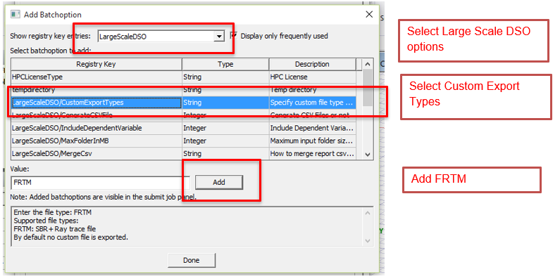
• When examining range-doppler problems, the SBR+ solver produces its raw data in a proprietary file format with the extension “.frtm”. You have the option to export these files for local solves through Export on Completion option in the Design Settings and for DSO parametric solves by specifying a batch option through the Job Management interface for Large Scale DSO. The relevant batch option for a DSO parametric solve for a range doppler problem is FRTM, as follows:
  

Using SBR+ Solution Type for HFSS SBR+ Range Doppler Designs

1. Moving Objects: Create or obtain 3D Components for any moving objects you intend to include in the scene as scattering geometry. These should be created within an HFSS Design set to the SBR+ Solution Type.

Stationary Objects: These can be 3D Components, but they can also be defined directly in the HFSS range-Doppler design if preferred.

The 3D Component should include material definitions and boundary assignments for all surfaces and bodies that are consistent with an SBR+ simulation.

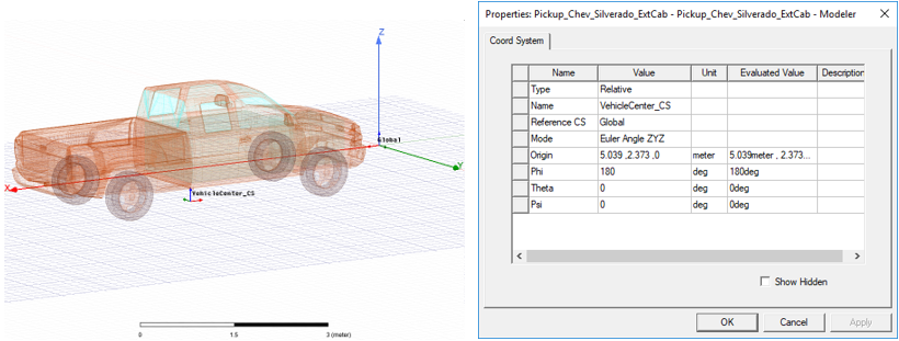
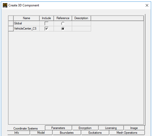
Choose a reference coordinate system that is convenient for the placement of the object within the larger scene. For example, with vehicles to be placed on the ground, it is convenient to define a local coordinate system that is laterally centered within the vehicle, with the z=0 plane at the bottom of the vehicle wheels, and oriented for forward travel in the +x direction. Be sure to include this local coordinate system definition and also select it as the reference coordinate system when the 3D Component is created.

2. Create a new HFSS Design for the radar scenario and set its solution type to SBR+.
3. Create a time variable that will drive the motion of all objects in the scene, including the radar antennas.

In the Project tree, right-click on the design node and select Design Properties…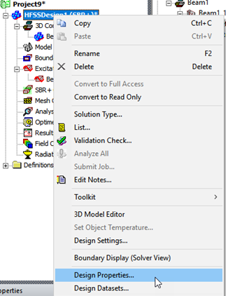

In the Properties dialog that appears, click Add…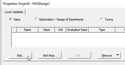

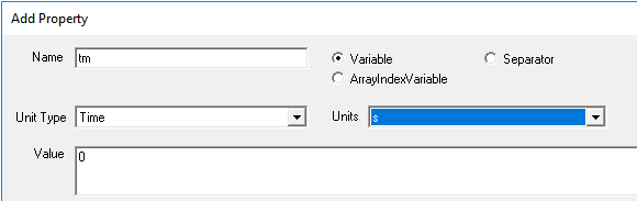
In the Add Property dialog that appears, set the Name to “tm” (or whatever you prefer to call the time variable) , select the property type as Variable, select the Unit Type as Time, and select a time unit (e.g., “s” for seconds).

Leave its Value as 0. You can later change it to advance the scenario or base its behavior on another variable through an expression in the variable definition.

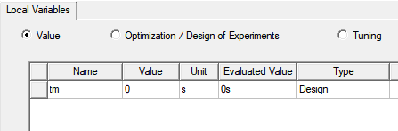
OK the dialog box. The new time variable is listed in the Design Properties.

4. Optional: Create or import geometry for stationary objects in the scene and assign boundaries to their surfaces.

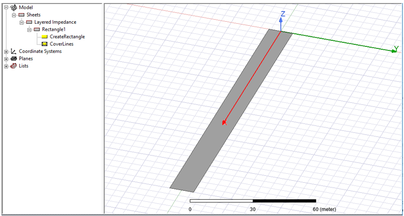
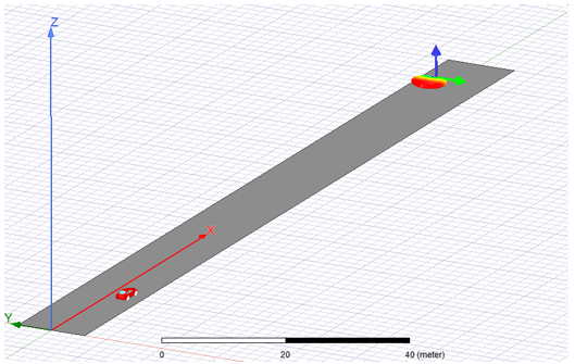
In this example, we’ve created a 150 m x 12 m rectangle to represent a road surface.

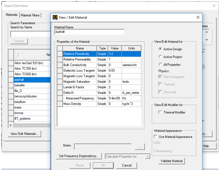
The material, “asphalt” has been added to the materials library, defined with a dielectric constant e_r = 3.2 and loss tangent tand = 0.03.

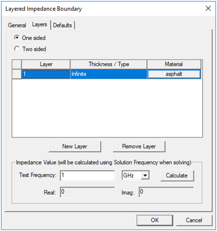
The assigned boundary is Layered Impedance: one-sided, one layer of “asphalt” with Infinite thickness. Because it is one-sided, it behaves as an asphalt half-space; SBR rays incident upon it will generate attenuated reflection rays but no transmission rays, with some energy lost to the half-space region.

5. Import 3D Components for moving scattering geometry and configure their time-dependent motion.

Optional: Create variables that define motion behavior. This will simplify the subsequent definition of coordinate systems. Here, for a vehicle, we specify:

• initial position: (Car1_x0, Unit Type = Length, Unit = meter),
• initial velocity: (Car1_vx0, Unit Type = Speed, Unit = m_per_sec),
• constant acceleration: (Car1_accel, Unit Type = Acceleration, Unit = m_per_s2).

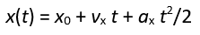
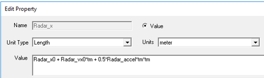
These variables are then used in an expression for a fourth Car variable that depends on the time variable (tm) for the x-position (Car1_x, Unit Type = Length, Unit = meter) of a coordinate system that will carry the 3D Component for a car in the scene:

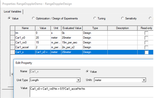
Verify correct entry of the expression for Car1_x by adjusting the input Value for the tm variable in the properties table and observing the Evaluated Value of Car1_x.

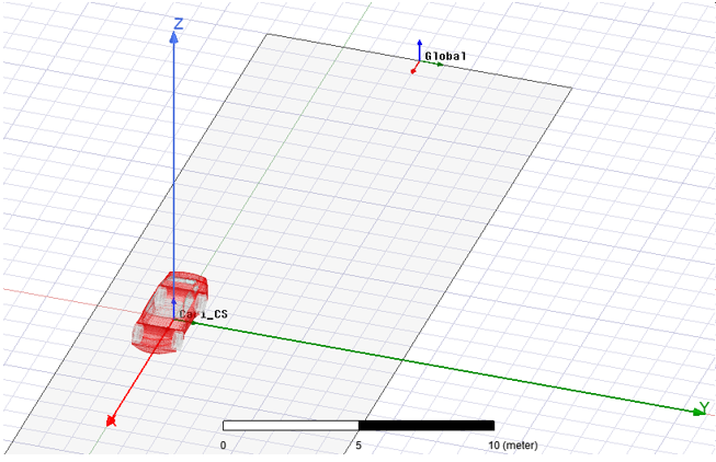
You then create a target coordinate system for the 3D Component: Car1_CS.

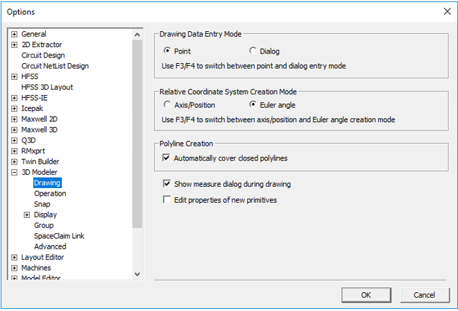
To follow this example, set the Relative Coordinate System Creation Mode to “Euler angle” in user preferences: click Tools >Options>General Options…, and then expand the 3D Modeler options group and select the Drawing options sub-group.

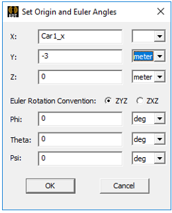
From the Toolbar menu, click Modeler>Coordinate System>Create >Relative CS>Both.

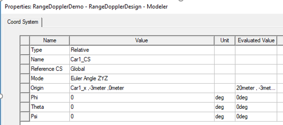
In the Set Origin and Euler Angles dialog box, set the X value to the Car1_x variable that you defined earlier and set the Y value to -3 m.

The created coordinate system is given a default name like RelativeCS1.

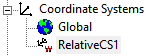
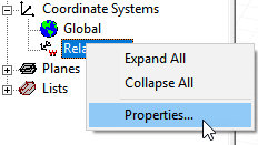
To access its properties and rename it, expand Coordinate Systems node in the History tree, right click on the newly created coordinate systems, and select Properties…

Rename it to Car1_CS in the Name field.

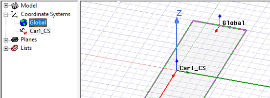
OK the dialog to show RelativeCS1 renamed as Car1_CS.

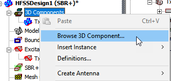
To import a 3D component, right-click the 3D Components icon in the Project tree of the range-Doppler design in the project tree and select Browse 3D Components…

Use the resulting file browser to select the 3D Component file (*.a3dcomp) of an object to include in the scene and click Open.

In the Insert 3D Component dialog that appears, select Car1_CS as the target coordinate system. This will cause the reference coordinate system of the 3D Component (see Step 1) to be fixed to and move with Car1_CS.

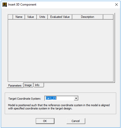
Click OK to insert your model at the Car1_CS. If your adjust the time variable, the imported component moves with Car1_CS.

6. Create and configure radar antennas.

Create a moving coordinate system for the radar antennas.

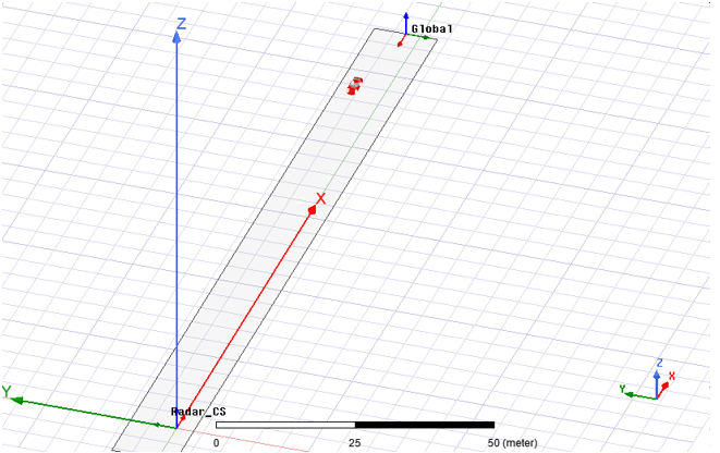
Below, we have defined Radar_CS relative to Global coordinates.

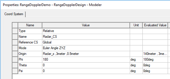
Its X component is set to a variable, Radar_x, which itself is defined in terms of other variables. Radar_x0 = 140 m, and Radar_vx0 = -15 m/s, Radar_accel = 0, and the time variable tm.

Its Y and Z components are set to 3 m and 0.5 m, respectively, the latter to elevate the radar antennas above the road.

By setting Phi = 180^o, we’ve oriented its X-axis to point in the -X direction of global coordinates.

Make the radar coordinate system (Radar_CS, in this example) the working coordinate system by selecting it in History tree. The working coordinate system becomes the target coordinate system of the radar antenna created in the next step.

Create the radar transmitting (Tx). A good choice for radar antennas is the built-in parametric beam, which example we will follow here. Alternatively, you can setup a link to a source design or import far-field gain pattern (.ffd) file. In the case of a one-way link from a source design, the Range-Doppler Setup Type only supports far-field links.

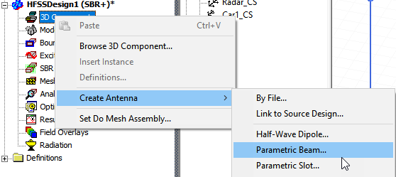
To create a parametric beam antenna, right-click on the 3D Components icon in the Project tree for the range-Doppler design and select Create Antenna>Parametric Beam…

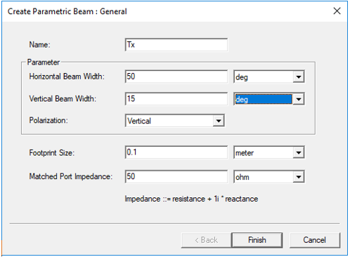
In the Create Parametric Beam dialog that appears, configure the beam widths and polarization. In this example, we have renamed the antenna to Tx. Then click Finish and the SBR+ source is created.

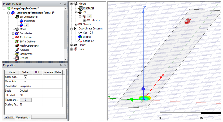
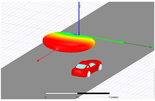
The following dialog shows the Project tree and History tree for the RangeDoppler demo with the 3D Components for car and antenna, and the coordinate systems.

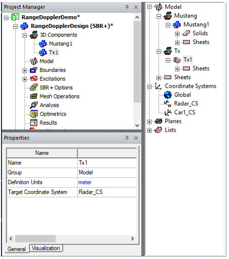
To increase the display size of the beam pattern to better match the scale of the scene, select the antenna’s object instance in the Project tree or History tree (Tx1 in this example), select the Visualization tab in the Properties window, and then adjust the Scaling Factor property as needed. Here, we have set Scaling Factor to 50.

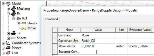
Create at least one radar receiving (Rx) antenna. In this example, we configure the Rx antenna as a vertically polarized parametric beam, but this time with a horizontal beam-width of 70^o instead of 50^o and naming it “Rx”. So that it moves with Tx1 antenna, we set its target coordinate system to also be Radar_CS. A move operation is then applied to the antenna instance (Rx1) to shift its position horizontally 2 cm relative to Tx1 (and the origin of Radar_CS). For a radar operating at 76.5 GHz (next step), this is a typical displacement between Tx and Rx antennas.

To effect the move operation to separate the Tx and Rx antennas:

• Select the Rx1 instance under the Rx definition node in the History tree.
• Select the Draw ribbon at the top of the main window.
• From the Operations group in the Draw ribbon, select Move.
• Press function key F4 to use dialog entry mode.
• Enter the Move Vector as 0, 0.02, 0 m. This will shift Rx1 by 2 cm along the Y axis of Radar_CS.

7. Configure Tx and Rx roles of antennas and port coupling pairs.

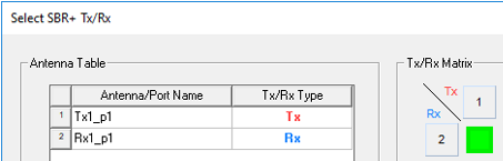
After all radar antennas and ports have been defined, configure which ports attach to transmitting (Tx) antennas and which to receiving (Rx) antennas. By default, the SBR+ solution type will compute the S-parameter coupling in both directions for each port pair. Unless all of these results are actually wanted, this causes wasted computational effort. Instead, use the Select SBR+ Tx/Rx dialog to select the particular coupling paths to be simulated. In the above example, where we only have two antennas, Tx1 and Rx1, and assuming we only want to transmit on Tx1 and receive on Rx1, meaning SBR rays will be launched only from Tx1 and their scattered field only observed on Rx1, the setup steps are as follows:

In the range-Doppler design, expand the Excitations node and notice it has two ports: Tx1_p1 and Rx1_p1.

Right-click on the Excitations node and choose the menu item, Select Tx/Rx… .The Select SBR+ Tx/Rx dialog appears. The Antenna Table on the left side of the dialog identifies the port names and assigns them an integer port Index: Tx1_p1 = Port 1, Rx1_p1 = Port 2. It also lists the potential role (Tx/Rx Type) of each port: Tx/Rx, Tx, or Rx. By default, each port has a Tx/Rx role, which means it can potentially act as both a transmitter and receiver. The Tx/Rx Matrix on the right side of the same dialog identifies which port coupling combinations are actually active. Tx-capable ports (that is, those with a role of Tx or Tx/Rx) are listed by index left-to-right across the top of the matrix. Rx-capable ports are listed by index top-to-bottom along the left side of the matrix. Active coupling paths are indicated by green squares in the matrix. By the default, all port pair combinations S_ij that are allowed by the assigned port roles are active, with the exception of self-coupling (that is, S_ii). In this example, we see that both S₁₂ and S₂₁ will be computed.

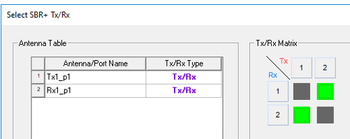
To switch off S₁₂, which means transmitting on port Rx1_p1 and receiving on port Tx1_p1, click on the corresponding (upper-right) square to turn it grey. This leaves only S₂₁ active.

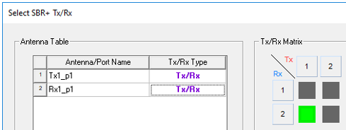
Alternatively, when there are many antennas and ports, and the matrix would grow large, it can be convenient to limit the roles of some ports. In this case, we can set Tx1_p1 to the role of Tx and Rx1_p1 to the role of Rx. This reduces the matrix to a 1 x 1, with a single green cell. Reducing port roles when they are known to be exclusively Tx or Rx for a particular system is especially helpful for MIMO radars with a large number of ports.

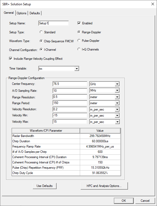
8. Configure the Range-Doppler Setup Type.

Right-click on the Analysis icon in the Project tree and select Add Solution Setup…

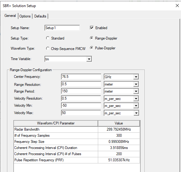
In the SBR+ Solution Setup dialog that appears, set Setup Type to Range-Doppler. This lets you select a Waveform Type of either Chirp-Sequence FMCW (default) or Pulse-Doppler. The simulation results (range-Doppler images) for Pulse-Doppler do not include the range-velocity coupling effect inherent in chirp-sequence FMCW (CS-FMCW). This effect is a shift in the perceived range of scattering features that is proportional to their radial (Doppler) velocity. The following figures show the Pulse-Doppler selection and configuration.

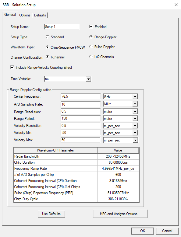
Selecting Chirp-Sequence FMCW offers additional options and settings: Channel Configuration (I-Channel or I+Q Channels), A/D Sampling Rate, and whether the waveform model should Include Range-Velocity Coupling Effect. See Chirp Sequence FMCW for SBR+ Range Doppler Solution Setup for further detail on configuring this waveform option and its range-velocity coupling effect.

Select the Time Variable. In this example, it is tm. Setting the Time Variable cannot be deferred.

Configure the Center Frequency and Range-Doppler performance specifications of the radar. This configuration will be applied to all port combinations selected in Step 7. When setting the Range-Doppler performance properties, there are several things to consider:

• Through the combination Center Frequency, Range Resolution, and Range Period, you are indirectly configuring a uniform frequency sweep. The Center Frequency (f_c) needs to be high enough to accommodate the Radar Bandwidth (BW) implied by the Range Resolution (Rr), which is obtained by the formula BW = c / (2 R_r), where c is the speed of light. The setup requires f_c > BW/2. For example, with a Range Resolution = 1 m, the frequency bandwidth is BW ~= 0.15 GHz. This means the Center Frequency needs to be 75 MHz or higher. Note that at the default frequency of 76.5 GHz, a Range Resolution of 1 m is easily accommodated. The number of frequency samples (N_f) in the implied sweep is then obtained as Range Period (P_r) divided by Range Resolution: N_f = P_r/R_r.
• The range response is periodic and, thus, ambiguous. If the Range Period is set to 100 m and a feature is observed at 40 m, this could mean the scattering feature is physically located 40 m from the radar, but in theory it could be 140m, 240 m, etc. from the radar. In radar data sheets, the range period is sometimes given as maximum range or range ambiguity.
• The Doppler velocity response is also periodic (and ambiguous). The Doppler velocity period P_v is determined from the dialog inputs as P_v = Velocity Max – Velocity Min. Suppose Velocity Min = -50 m/s and Velocity Max = 70 m/s. This means the reported Doppler velocity period is Pv = 120 m/s, centered at 10 m/s. Suppose a scattering feature is observed to have a Doppler velocity of 50 m/s. In theory, this could mean its actual Doppler velocity relative to the radar is -70 m/s, +50 m/s, +170 m/s, or any other value of 50 m/s + n 120 m/s, where n is an integer. In radar data sheets, the Doppler velocity period is often expressed through a minimum and maximum velocity, but it can also appear directly as the velocity ambiguity or period. With range-Doppler radars, the ambiguous (periodic) quality of range and velocity is an unavoidable design limitation.
• There is a tradeoff between range and velocity ambiguity. In general, the higher the range ambiguity (period), the lower the maximum theoretically achievable Doppler velocity ambiguity (period), and vice versa. The input dialog for the Range-Doppler setup will not permit a violation of this theoretical limitation, as it would then result in a meaningless range-Doppler performance specification that is not physically realizable in any radar. The constraint is given by the following inequality:

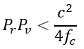
In this example, we select the following range-Doppler settings:

• Center Frequency = 76.5 GHz
• Range Resolution = 0.5 m
• Range Period = 150 m
• Velocity Resolution = 0.5 m/s
• Velocity Min, Max = -50, 50 m/s

Select the Options tab to set the SBR+ Solver Options: Ray Density and Maximum Number of Bounces.

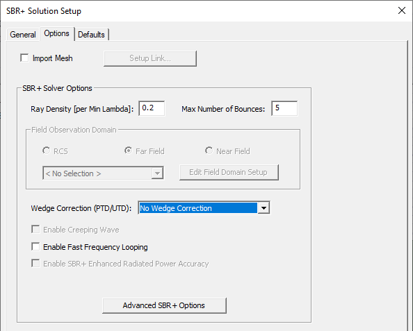
Note that the default Ray Density for the Range-Doppler Setup Type is 0.2 rays/wavelength whereas its default for the Standard Setup Type is 4.0 rays/wavelength. The lower default Ray Density for the range-Doppler setup reflects the fact that it is optimized for millimeter-wave radars operating in scenes spanning hundreds of meters (typically tens of thousands of wavelengths). For example, at the default center frequency of 76.5 GHz, the wavelength is 3.9 mm. A ray density of 0.2 rays/wavelength therefore corresponds to a first bounce ray-spacing of about 2 cm. Unlike matrix-based solutions, SBR has no inherent requirement for sub-wavelength sampling of the scattering geometry. Rather, it is sufficient if the rays adequately sample the geometric features of the scatterer irrespective of wavelength. For this example, we use the default SRB+ Solver Options: Ray Density = 0.2 rays/wavelength and Maximum Number of Bounces = 5.

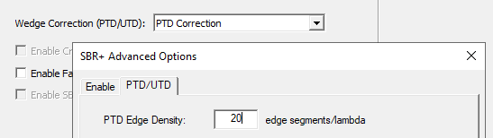
Wedge Correction can be selected from the dropdown for PTD and UTD. When two different bodies (with different body IDs) with possibly different velocities join during a simulation to form a valid wedge, the two sides of the wedge are treated as knife wedges. Wedges are extracted as expected for triangles belonging to the same body. For example, imagine two separate plates moving towards each other that at time t join to form a dihedral. The extracted wedges will be two distinct knife edges rather than one dihedral wedge. If you select PTD Correction or PTD Correction + UTD Rays, the Advanced SBR+ Options includes an option to Enable PTD/UTD (Wedge Diffraction) options. You can then specify PTD Edge Density as edge segments/lambda.

The Enable Fast Frequency Looping (FFL) option is available for range-Doppler setups. FFL will significantly accelerate a range-Doppler simulation in most cases, usually with little loss of fidelity. FFL accelerates high-density frequency sweeps with uniform frequency intervals. All range-Doppler setups imply uniform frequency sampling and typically also require a large number of frequency samples to achieve a Range Period spanning many Range Resolution intervals. FFL begins to show significant speed-up when the number of frequency samples exceeds 10, improving to 5x – 10x or greater when the number of samples exceeds 100. The number of frequency samples of your setup can be determined by consulting # of Frequency Samples (for Pulse-Doppler) or # of A/D Samples per Chirp (for Chirp-Sequence FMCW) in the table at the bottom of the General tab of the setup dialog box. Typical range-Doppler setups also have a relative bandwidth (Radar Bandwidth divided by Center Frequency) well under 10%, making them ideal for the accuracy of FFL acceleration. See SBR+ Fast Frequency Looping for High-Density Sweeps for details on the benefits and limitations of this acceleration feature.

9. Advanced Option for Geometrical Optics (GO) Blockage

SBR+  normally applies a physical optics (PO) blockage model where blockage effects emerge from partial cancellation of the incident field by the scattered field. PO blockage not only occurs in connection with the incident field from the Tx antennas, but also within the scattered field itself when reflected fields from the previous bounce are diminished by a blocking surface along the geometrical-optics (GO) reflection path at the current bounce by evaluating the scattering contribution of the incident ray field at that bounce.

In cases of significant blockage by a large obstruction, the PO blockage model requires accurate currents over the extent of the obstruction. Sometimes, this is hard to achieve in the ray tracing approximation. For example, the obstruction may not be well illuminated by direct rays from the Tx antenna or multi-bounce rays after an earlier reflection. An alternative is to use a GO blockage model where scattered field contributions are added to an observation point subject to a line-of-sight (LOS) blockage check performed by the ray tracer. In some cases, this is more accurate than the default PO blockage formulation, while in others it is less accurate. GO blockage also entails a non-trivial computational cost, as the blockage check with the ray tracer must be performed for each observation angle (or point) for each ray hit point.

In addition to GO Blockage for SBR and UTD ray tracks, this feature is also available for PTD and CW.

Limitations:

GO Blockage formulation is suited specifically for SBR+ ray tracks, including UTD ray tracks. While GO Blockage for CW and PTD has been implemented for the first time in this release, results can be surprising and/or inaccurate, as a limitation of the methodology.

Summary Workflow:

GO Blockage works with every SBR+ modality, in Hybrid and SBR+ solution type, with any type of source (plane wave vs antenna), and even in ADP mode.

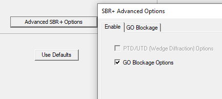
Click the Advanced SBR+ Options button to open the SBR+ Advanced Options window. On the Enable tab, Check GO Blockage Options to enable the GO Blockage tab.

On the GO Blockage tab, you have check box options to enable or disable GO Blockage and enable or disable Surface Self-block.

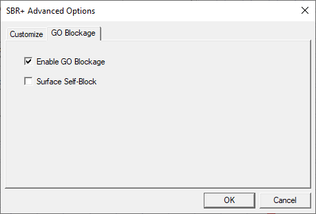
Surface Self-Block: if enabled, the surface where the footprint is radiated from is used for blockage check, that is, anything below the surface wrt respect to the incoming ray is not in line of sight. If the setting is disabled, the footprint surface is not used for blockage checks (anything below the surface wrt the incoming ray is in line of sight), but other surfaces are used for blockage.

10. Generate Range-Doppler report.

After validating the solution setup and executing the analysis, you can generate a range-Doppler image for each configured port-coupling pair by right-clicking on the Results icon in the Project tree and selecting Create Range-Doppler Report>Rectangular Color Map Plot or select the Results tab of the ribbon and click Range-Doppler Report>2D Color Map.

In the Report dialog that appears, first configure the post-processing settings.

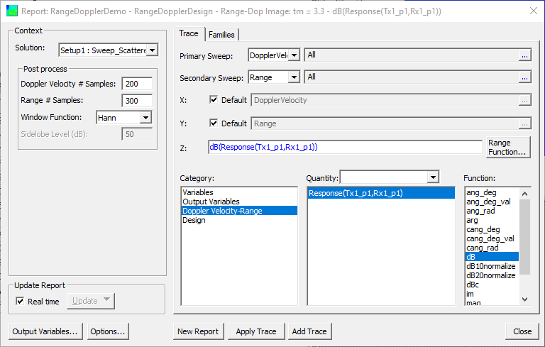
The width and height of the image in pixels is set by Doppler Velocity # Samples and Range # Samples, respectively. By default these correspond to the settings in the Range-Doppler setup. For example, since the Velocity Min and Max were -50 m/s and +50 m/s, this means the velocity period is Pv = 100 m/s. The Velocity Resolution was set to Rv = 0.5 m/s. Therefore, the default number of Doppler velocity samples is Pv/Rv = 200. Similarly, the Range Period and Range Resolution were set to Pr = 150 m and Rr = 0.5 m, respectively. Therefore, the default number of range samples is Pr/Rr = 300. The default number of samples preserves all information but the results might appear choppy. You can increase or decrease the number of samples (image pixels) relative to the default to either over-sample or under-sample the image. Over-sampling smooths out the image without adding information, while down-sampling causes information to be lost. In this example, we stick with the default number of samples.

The Window Function selection controls the tradeoff between feature blurring and signal-processing sidelobe suppression. There are four options: Hann (default), Flat, Hamming, and Taylor.

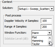
In radar imaging applications, Hann provides a good compromise between blurring and sidelobe suppression. The Flat window provides the best resolution (no blurring), matching the range and velocity resolution specifications in the Range-Doppler Setup. However, its first sidelobe is only -13.3 dB down from the feature peak, and subsequent sidelobes decay slowly. This means the sidelobes of strong features in the image tend to mask weaker ones. The Hann (aka Hanning) window has a first sidelobe that is -31.5 dB down from the feature peak, and subsequent sidelobes decay quickly from there, but the achieved resolution is twice as large (blurry) as that specified in the Range-Doppler Setup. The Hamming window has very similar resolution to the Hann window, and its first sidelobe is -42.7 dB down from the feature peak, which is better than Hann. However, subsequent sidelobes decay very slowly from there, so strong features in the image have a greater tendency to mask weak features compared to the Hann window. The Taylor window provides the option to customize sidelobe levels, and the specified level will be roughly identical for all sidelobes. As with the other window functions, the higher the sidelobe suppression that is configured for Taylor, the greater the amount of blurring. In this example, we stick with the default Hann window.

• Under the Trace tab, leave the Category selection as its default: Doppler Velocity-Range.
• Under the Quantity label, select the port-pair combination to display. In this example, there is only one option: Response(Tx1_p1,Rx1_p1).
• The range-Doppler image is complex-valued pixels. Select the Function to apply to the complex data in order to convert it into a real number that can be mapped to a linear color map. The default Function is dB. This is recommended for most cases since typically a large dynamic range is required to simultaneously observe multiple features.
• Click the New Report button to generate the range-Doppler plot.

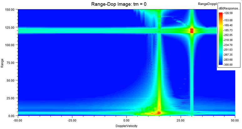
Because the default color map has a lower extent of -300 dB, while the strongest feature (that of the oncoming car) has a peak strength of ~-129 dB, the descending sidelobes of the Hann window are evident across the range and Doppler velocity extents of the image.

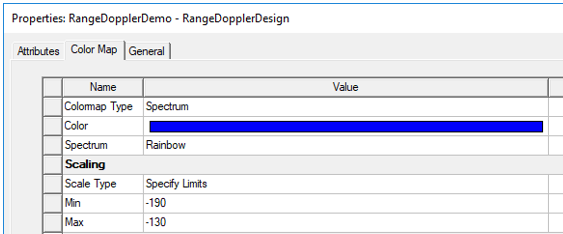
To customize the scale of the color map, double-click on the color map legend.

In the Properties dialog that appears, select the Color Map tab. Under the Scaling group, change the Scale Type from Auto Limits to Specify Limits and then enter the Min and Max dB values of the color map. In this example, we set Min and Max to -190 and -130 dB, respectively.

By default, the number of colors in the color map is 64. To achieve round numbers in the labeling of the color bar, you need to set Value Type to Specify Num. Levels (default) and set Num. Levels (N_lvl) according to the dB span (S_dB) of the color map. To achieve a fairly continuous color map, N_lvl >= 50 is recommended. Beyond that, choose N_lvl so that S_dB/(N_lvl – 1) is a round number like 0.5, 1, or 2 dB. In this example SdB = -130 dB - (-190 dB) = 60 dB. Thus, we choose N_lvl = 61.

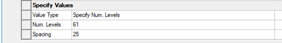
This results in a color map with labels at precisely 4 dB intervals.

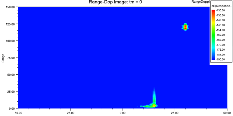
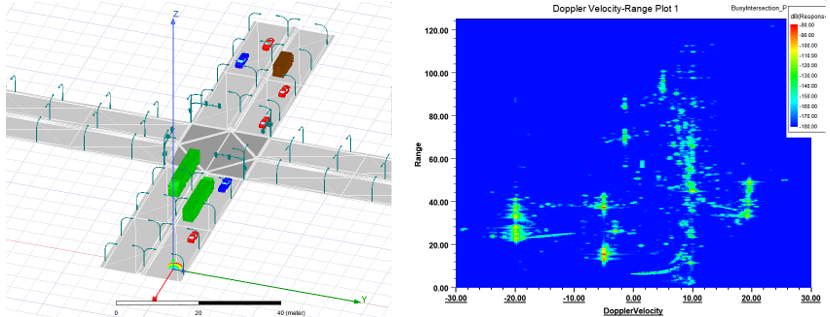
The following image is generated for time tm = 0, when the velocity of the car is 15 m/s in the +X direction and the velocity of the radar is 15 m/s in the -X direction. Also, the position of the car is X = 20 m while the position of the radar is X = 140 m. Thus, we observe a range-Doppler feature at range 140 – 20 m = 120 m and velocity 15 - (-15) m/s = 30 m/s. Notice also that the response of the car is spread out in range because the car is an extended object spanning roughly 5 m. There is also a smeared feature near range = 0 m and velocity = 15 m/s. This represents the return from the road as filtered by the Tx and Rx beam antennas of the radar.

With this setup, you can generate results for any value of time tm. Below we have advanced time to tm = 3.3 s.

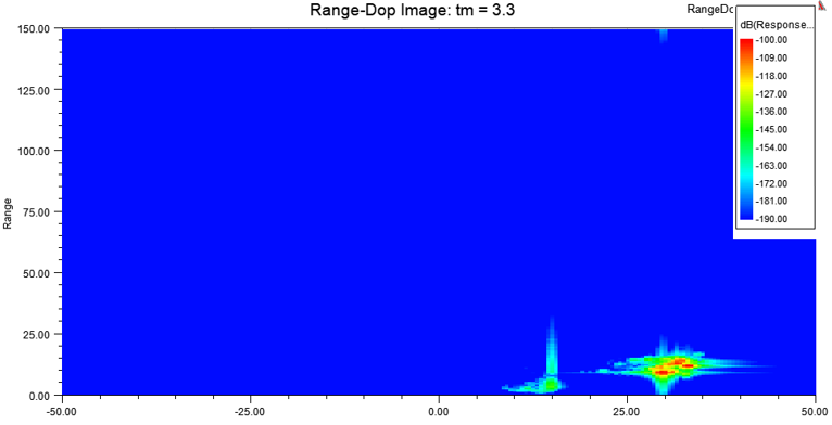
At this point in time, the car is about to pass by the radar.

The car is traveling 21.6 m/s in the +X direction while radar remains traveling at 15 m/s in the -X direction. Thus, we might anticipate a Doppler velocity of 36.6 m/s. However, only the radial component of the velocity between radar and the car is captured in Doppler velocity. To determine that, we need to consider the position of the car relative to the radar. At tm = 3.2 s, the center of the car is located at (80.4, -3, 0) m while the radar is located at (90.5, 3, 0.5) m in global coordinates. Relative to the Radar_CS coordinate system, the velocity vector is (-36.6, 0, 0) m/s while the displacement vector from the radar to the car is (10.1, 6, 0) m. Because of the finite vertical extent of the car, we assume the vertical (Z component) displacement from the radar to the car is zero. Thus, we anticipate a feature with a Doppler velocity of 31.5 m/s and a range of 11.7 m. This is consistent with the resulting range-Doppler image shown above (note we have changed the color map to now extend from -190 dB to -100 dB). However, notice that the observed Doppler velocity is spread out between roughly 29 m/s and 34 m/s whereas at tm = 0, the observed Doppler response was more tightly confined about the anticipated Doppler velocity of 30 m/s. At this close proximity to the radar, the front and rear of the car subtend a significant angular span relative to the radar, and this causes a corresponding spread in the observed Doppler velocity response.