Selecting the Solution Type 

Before you draw the model for an HFSS project, specify the design's solution type. As you set up your design, options available in the user interface will depend upon the selected solution type.

1. Click HFSS>Solution Type.

The Solution Type dialog box appears.

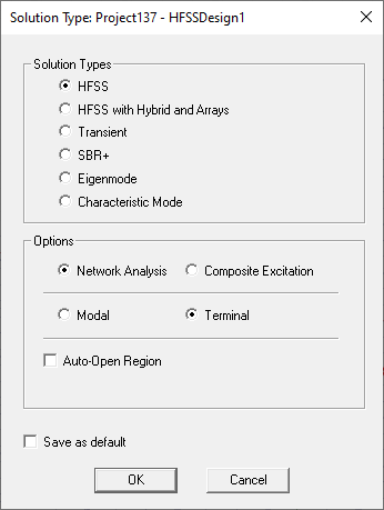
2. Select one of the following solution types:
   

   Solution Types
   HFSS	This enables the Driven Options Modal and Terminal (the default). HFSS selection enables Mesh Fusion for FEM components. You can add padding to the mesh bounding volume. The finite array is disabled, and the Hybrid folder is removed from the project tree. The FEBI boundary becomes a regular boundary instead of hybrid region. When there are components set up for mesh fusion, the solution setup only allows direct solver and no derivatives.
   HFSS with Hybrid and Arrays	This enables the Driven Options Modal and Terminal (the default). HFSS with Hybrid and Arrays selection enables mesh assembly for hybrid components. Users cannot add paddings to the mesh assembly bounding volume. The finite array is enabled, and the Hybrid folder is added to the project tree, along with the tab for Hybrid in the solution setup.
   Transient	For calculating problems in the time domain. It employs a time-domain ("transient") solver. For Transient your choice of Composite Excitation or Network Analysis affects the options for the setup. If you select Network Analysis the setup includes an Input Signal tab for the simulation. Typical transient applications include, but are not limited to: Simulations with pulsed excitations, such as ultra-wideband antennas, lightning strikes, electro-static discharge; field visualization employing short-duration excitations; time-domain reflectometry.
   SBR+	This option simplifies design creation for SBR+ users. HFSS can use EMA3D shooting and bouncing ray (SBR) technology to calculate the far field from current sources and defined geometry via a one-way coupling. With this solution type, you do not need to specify explicit SBR+ Hybrid Regions. The Driven option for this solutions is Network Analysis only, with no Auto-Open Region. For details, see Design Flow for SBR+ Solution Type. You can also use parametric antennas in SBR+ solutions. For SBR+ solutions, you see an option in Initial Mesh Settings to Allow tolerant meshing in SBR+ regions. For HFSS SBR+solutions, you can also choose to import STL files as Lightweight Geometry.
   Eigenmode	For calculating the eigenmodes, or resonances, of a structure. The Eigenmode solver finds the resonant frequencies of the structure and the fields at those resonant frequencies. Eigenmode designs cannot contain design parameters that depend on frequency, for example a frequency-dependent impedance boundary condition.
   Characteristic Mode	This option is used for calculating the characteristic modes of a structure. The structure can be metal or dielectric. The solution reports the Number of Modes, the characteristic angle and current (amp/meter), the modal significance and quality factor, and the voltage per port based in edit sources weighting. Selecting Characteristic Modes changes the Solution Setup criteria and dialog. You specify the minimum modal significance (default 0.02). Convergence is based on Max E rather than Max S (default (0.02). Only discrete sweeps are supported. Only the CMA solver is supported. Only lossless boundaries are allowed. Finite conductivity boundaries are allowed but are converted to lossless. The half-space boundary is not allowed. Related Topics: Theory of Characteristic Mode Analysis Edit Sources Panel for Characteristic Mode Analysis Generating Reports for Characteristic Mode Analysis

   
   

For the Driven Solutions, specify whether to use Network Analysis or Composite Excitation. Network Analysis is the default for driven problems. Composite Excitation provides a method for solving fields in a large frequency domain problem.

3. For HFSS Driven solutions, you can select a range of Driven options.
   

   Driven Options
   Modal	For calculating the mode-based S-parameters of passive, high-frequency structures such as microstrips, waveguides, and transmission lines which are "driven" by a source, and for computing incident plane wave scattering. Network Analysis is the default and functions as before. Composite Excitation provides a method for solving fields in a large frequency domain problem. See Assigning Wave Ports for Modal Solutions and Assigning Lumped Ports for Modal Solutions.
   Terminal	For calculating the terminal-based S-parameters of passive, high-frequency structures with multi-conductor transmission line ports which are "driven" by a source. Terminal is the default. This solution type results in a terminal-based description in terms of voltages and currents. Some modal data is also available. Network Analysis is the default and functions as before. Composite Excitation provides a method for solving fields in a large frequency domain problem. See Assigning Wave Ports for Terminal Solutions and Assigning Lumped Ports for Terminal Solutions.
   Network Analysis	Network Analysis is the default and functions as before.
   Composite Analysis	Composite Excitation provides a method for solving fields in a large frequency domain problem.
   Auto-Open Region	For open region problems (typically antennas), you can choose Auto-Open Region. The option is available for Driven modal, terminal and transient solution type. This automatically creates an open region and a predefined Analysis setup for the project. You can select whether the region is Radiation, FE-BI, or PML. This simplifies the design process. If you do not choose Auto-Open Region, you must create an airbox and then assign a radiation boundary, either manually, or using the Create Open Region command. For more information on this Solution setting, see Using Auto-Open Region for the Solution Type for Antenna Designs.