Parametric Antennas for SBR+ Solution Type

For SBR+ solution type, you can access a range of parametric antennas. Parametric antennas are antenna sources that either have no physical structure definition or a highly idealized physical structure. No model parts are constructed or used in the simulation. They create far-field pattern or current distribution sources that can provide S-parameter outputs and composite far-field radiation patterns. The SBR+ solver will automatically interpolate the source fields from the file-based antenna in order to represent the antenna at all frequencies of the user defined frequency sweep in solution setup. The file-based antenna requires at least two frequencies, and the min/max frequencies of the user defined sweep should fall within the frequency band of the file-based antenna.

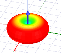
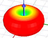
Parametric antennas are very quick to define and place, copy and duplicate, and are thus intended for systems studies where the specific antenna structure is either unknown or a simple, topologically representative antenna type is sufficient. The editable parameters depend on the antenna type. In the model window, the antennas display as a scaled far field pattern at the antenna origin. The model is listed under the Project tree under 3D Components and automatically includes a port to support S-parameter output. You can change port post-processing setting from the Properties window. Selecting the antenna causes the Properties window to display with tabs for General antenna Properties, and Visualization settings.

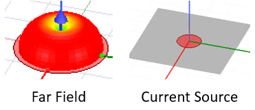
Several of the parametric antennas let you choose Antenna Representation as Far Field Source and/or as Current Source.

Other parametric antennas include only Current Source representation.

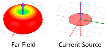
Current sources are visualized in the model window as a set of short lines with arrows to indicate the current direction. When placed near a geometric surface, these current sources can be configured to conform to the nearby surface. The current source conformance can be configured globally, to be enabled/disabled for all antennas in the HFSS design, or enabled/disabled for each parametric antenna or array.

For a technical discussion, see Current Conformance and Array Conformance in SBR+.

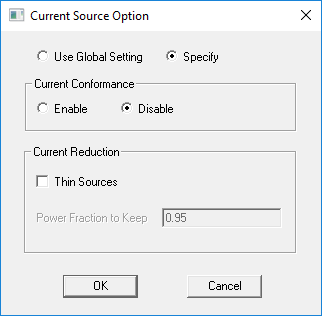
The Current Source Option window also includes Current Reduction option.

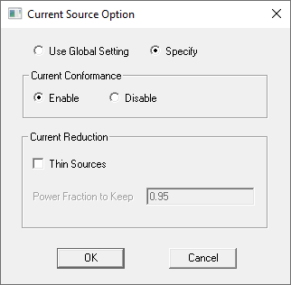
Enabling Thin Sources lets you specify a Power fraction. It should be greater than 0.1 and less than 1. Solutions are invalidated if you change current source conformance, use Thin Sources, Power Fraction, or change the Global option.

The outputs from SBR+ simulations with parametric antennas include:

• S-parameters.
• Composite far-field radiation patterns.
• Incident field reporter outputs provide the free space radiation patterns of the antenna.

Prerequisites

• The Solution Type must be SBR+.
• If you use a File-based parametric antenna, it must be defined with at least two frequencies whose min/max meet or exceed the extents of the simulation frequency sweep.

Adding Parametric Antennas

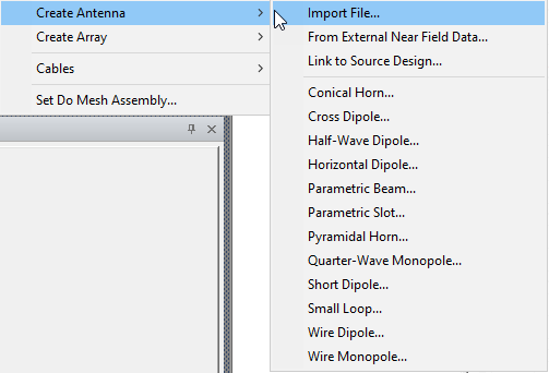
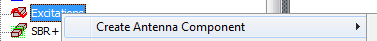
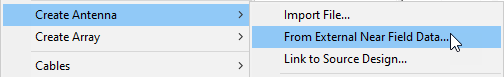
1. Right-click the 3D Component folder in the Project tree to see the Create Antenna menu:

You can also view the parametric antenna menu by clicking HFSS>Excitations>Create Antenna Component or by right-clicking on the Excitations icon and selecting the submenu under Create Antenna Component.

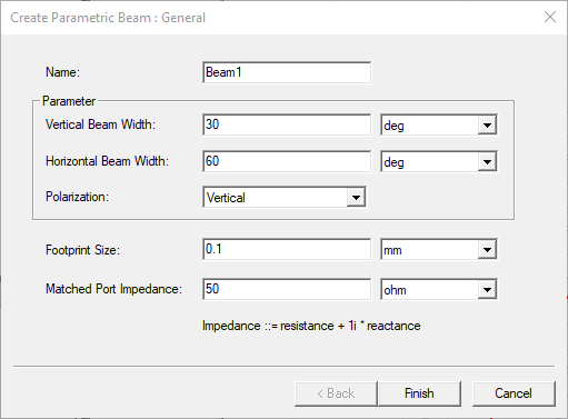
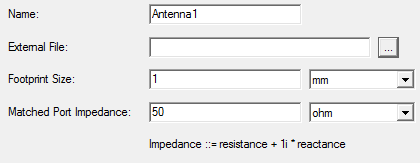
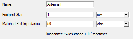
Selecting any of the pre-defined antennas causes a dialog to appear, which includes the name, and other parameters. For example, the dialog below shows the Create Parametric Beam dialog.

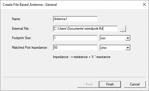
For the By File antenna, the Parameters include a path for a Far Field data file (*.ffd format).

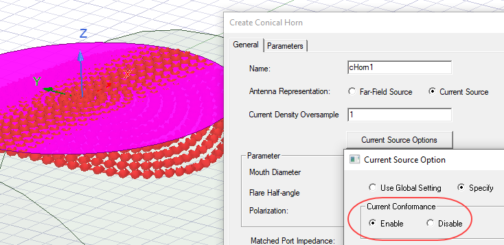
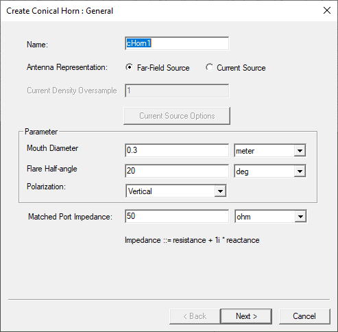
The Conical Horn dialog includes the option for representation as Far Field and/or Current Source.

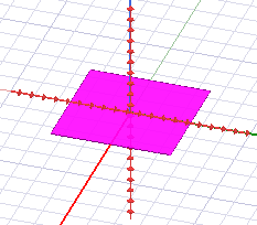
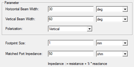
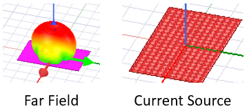
Depending on your selection, the visualization may appear as follows.

If the antenna offers current source, and you select that option, the Current Source Options button is enabled on the Create dialog box. Select it to open the Current Source Option. dialog.

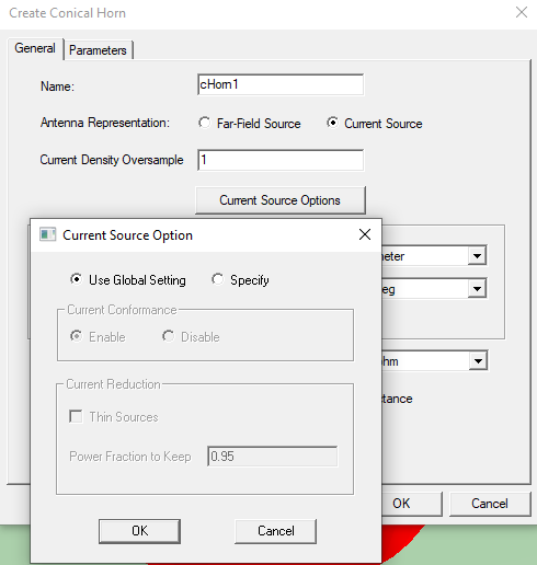
For the global current source options, see Set Current Source Option. To override the global setting, select Specify. This enables Current Conformance and Current Reduction settings for this antenna.

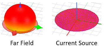
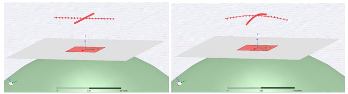
Current conformance controls whether antennas placed near a geometric surface conform to that surface. The figure on the left shows current conformance disabled. The figure on the right shows current conformance enabled.

Enabling Thin Sources lets you specify a Power fraction. It should be greater than 0.1 and less than 1. Solutions are invalidated if you change current source conformance, use Thin Sources, Power Fraction, or change the Global option.

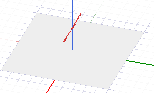
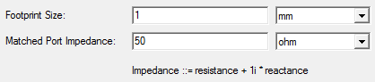
2. Specify the parameters as desired. The parametric antenna footprint is a visual to aid in placing and orienting the antenna, but it has no impact on simulation results.

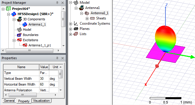
The antenna appears in the Model window.

3. If you want to edit the antenna placement, or orientation, select the model in the History tree, and right-click and select Edit>Arrange, and select from Move, Rotate, or Mirror.

You can also change or edit the target coordinate system in the instance Property window.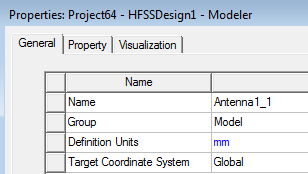

Notice that other edit commands for Copy, Paste, and Duplicate are also available.

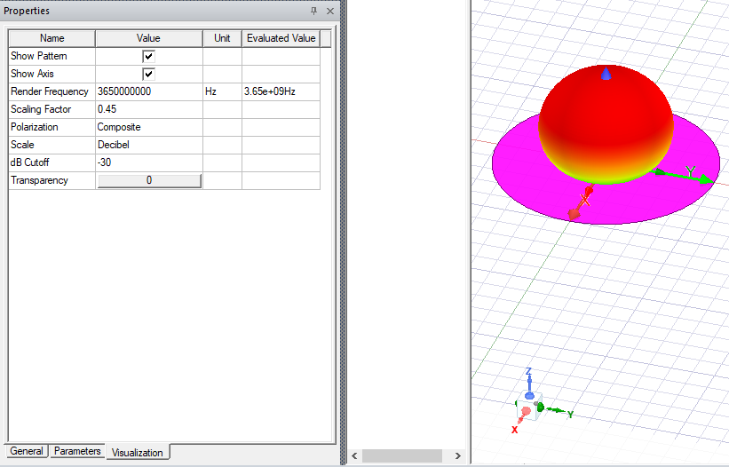
4. If you want to edit the Visualization parameters, select the Antenna model icon under the Project tree or History tree to view the Properties, and select the Visualization tab. The visualization parameters available can be different for different antenna models. Visualization parameters have no influence on simulation results. They only determine how the parametric antenna is displayed in the model viewer.
   

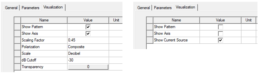
• Choose whether to show the pattern and/or axis. Parametric antennas in a current-sources representation also provide the option to view them according to their far-field Pattern, even though they always launch rays from a distribution of currents sources during SBR+ simulation.
• If the antenna parameters include Show Current Source, you can enable or disable visualization here.
• For Polarization, click on the cell for a drop-down menu selection for Composite, Horizontal, Vertical, LHCP, or RHCP. The Polarization rendering setting only controls which polarization component of the parametric antenna's radiation pattern is currently displayed. It has no impact on the polarization characteristics of the parametric antenna definition and, thus, no impact on simulation results. Some antennas, such as the Parametric Beam, also provide a control for its polarization behavior in the Property tab, which does influence simulation results.
• Scale can be Decibel (the default), Linear, or Power.
• dB Cutoff appears when you select Decibel as the Scale. This sets the dB level at the pattern display origin relative to its peak level.
• For Transparency, click on the cell for a dialog with a slider and text field.
• For Scaling Factor, click on the cell to edit the value. The Scaling Factor controls how large the antenna's radiation pattern is displayed relative to its Footprint Size.

5. After you run an SBR+ simulation with parametric antennas, you can create a variety of reports, including S Parameters, Far Fields, and Antenna Parameters.
   

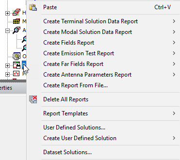
You must create a Far Field Setup to access the Far Fields and Antenna Parameters reports.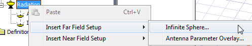

Parametric Antenna Descriptions

When you specify an SBR+ Solution type, you have access to the following sources and parametric antennas:

• By File Antenna for SBR+
• From External Near Field Data
• Link to Source Design
• Conical Horn (far field or current source option)
• Cross Dipole (current source)
• Half-Wave Dipole
• Horizontal Dipole (current source)
• Parametric Beam
• Parametric Slot (far field or current source option)
• Pyramidal Horn (far field or current source option)
• Quarter-Wave Monopole
• Short Dipole
• Small Loop
• Wire Dipole (far field or current source option)
• Wire Monopole (far field or current source option)

By File Antenna for SBR+

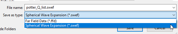
You define the By File... antenna by importing an external file containing far field data in .ffd, or for Spherical Wave Expansion Import, you can import .swef format files.

Pattern samples are entered over a two-dimensional angular sampling domain in spherical coordinates, θ and φ per frequency. The initial or final angle can be arbitrary (that is, no restriction on θ being from 0 to 180 degrees, and φ from 0 to 360 degrees). Nevertheless, the sampling of the θ and φ domain must be such that if adding more points to the domain, 0- and 180-degree samples are exactly captured.

For example, suppose one domain is defined as 1 90 90, that is, from 1 to 90 degrees with 1-degree step. This domain is compatible with the above restriction, because by adding points to the domain every 1 degree the domain can be extended to 0 180 181.

Consider another domain defined as 1 89 45, that is, from 1 to 89 degrees with 45-degree step. The domain is not compatible with the above restriction, because 0 and 180 degrees cannot be exactly sampled by continuing the domain. In other words, the external far-field can be specified over a sector which does not include θ = 0 or 180 degrees and φ = 0 or 180 degrees. However, if the defined sector is extended to cover the entire sphere using the specified sampling, the entire sphere should contain samples at θ = 0 and 180 degrees, φ = 0 and 180 degrees.

The SBR+ solver will automatically interpolate the source fields from the file-based antenna in order to represent the antenna at all frequencies of the user defined frequency sweep in solution setup. The file-based antenna requires at least two frequencies, and the min/max frequencies of the user defined sweep should fall within the frequency band of the file-based antenna.

Pattern levels specified in the file are automatically renormalized so the antenna radiates at the power level specified in the Edit Post Process Sources dialog.

For detailed information on the swef format, see Spherical Expansion Wave Source (*.swef).

For detailed information on the ffd format, see External Data File for Far Field Wave.

For editing properties, placement, and visualization, file based antennas resemble parametric antennas.

For the By File antenna, the Visualization tab for Properties also includes a drop down for Render Frequency which lists the available frequencies defined in the Far Field data file (*.ffd).

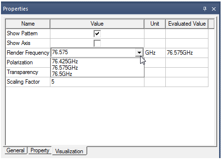
If you enable the Show Pattern, or load a design with the option enabled, if the .ffd file is not found, an error message reports this. Validation checks to see if the Render frequency specified is provided in the .ffd file. After you create a File Based Antenna, you have the option to reload the *.ffd file. If you archive a project with a File Based antenna, the process automatically includes the *.ffd file and restores it to a relative location for portability.

If you import of Spherical Wave Expansion File import for .swef files, visualization for the antenna is also available. Visualization parameters include Render Frequency, Scaling Factor, Polarization, Scale, dB Cutoff, and Transparency. You can edit fields or select from drop down menus. You can use an SWE antenna to produce S-matrix and far field results.

From External Near Field Data

Near field characteristic of the source antenna, which is saved in .and and .nfd format, can be used to create external near field antenna and act as a virtual port in SBR+ target design. Compared to near field antenna link, this "file-based" near field approach does not need any information of the source antenna design except for the near field on specific sample points, and is therefore convenient to use and easily maintainable and scalable.

For defining simple-primitive near field source, HFSS uses two kinds of external data file. First, the actual location/field data is stored in .nfd format. Second, the Ansys Near field Descriptor file (.and file) stores the general geometry information and paths of .nfd data. Adding a external near field link to HFSS design is therefore a two-steps workflow. During excitation setup, an external near field design (that is, a design with a box representing mesh points) is created based on information in a .and file and linked to target design. During simulation, external near field design acquires mesh points and field from .nfd file based on specific frequency the target design asks for.

For HFSS SBR+ design you can also create external near field design based on an .and file or select from existing ones. A virtual port is created for each external near field antenna, and its corresponding footprint is created similar to an HFSS linked antenna.

To create a new Near Field design, based on an .and file:

Open an empty SBR+ design, open external near field antenna dialog by selecting 3D Component > Create Antenna > From External Near Field Data...

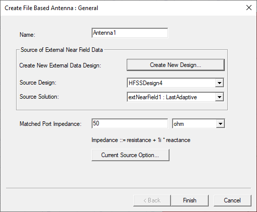
This opens the following Create File Based Antenna dialog:

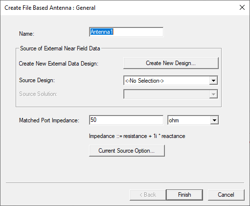
Initially, because there is no external near field design, the “Source Design” combo box shows “No Selection” and “Source Solution” combo box is greyed out.

To create a new external near field design, select the Create New Design... button. A file selection dialog will pop out and boundary type is allowed for selection.

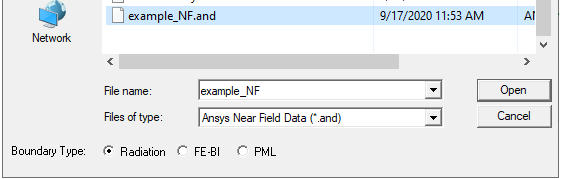
When you select an .and file, make the Boundary Type selection, and click open, the Create File Based Antenna dialog is populated with information about the Source Design and Source Solution.

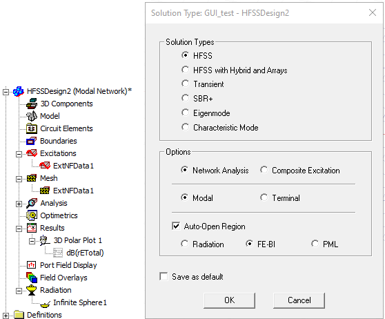
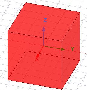
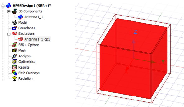
Additionally, a new external near field design (“HFSSDesign2”) is created in the Project tree. This newly created design automatically creates several setups like mesh, solution, report and radiation. It also creates a native geometry as defined in .and file.

The modeler window shows a native geometry as defined in the .and file.

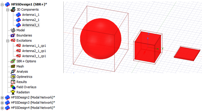
Click Finish in the Create File Based Antenna dialog and a new external near field antenna is created, together with a virtual port and antenna footprint (including outer bounding box and inner near field geometry).

Editing an existing external near field antenna

Let say we already create several external near field antennas and their corresponding external designs using similar approaches.

When we edit one of the antennas (in this case Antenna3), the dialog show its corresponding source design name and solution name.

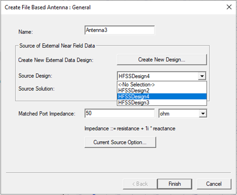
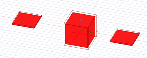
If we change the source design and click Finish, its footprint will be updated.

Link to Source Design

HFSS lets you create a one-way link from a Driven Modal or Driven Terminal design to an SBR+ design.

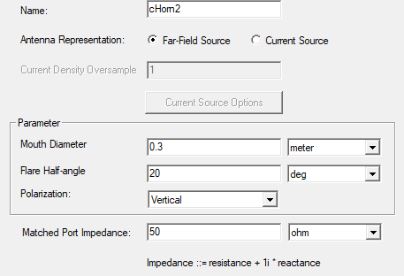
Conical Horn

This frequency-dependent antenna approximates a flared conical horn with user-defined dimensions and polarization. It is based on the approximated field distribution of a circular cross-section conical horn driven in the TE₁₁ waveguide mode. The model accounts for phase taper at the edges of the flat aperture (horn mouth) due to the spherical phase front introduced by the walls flaring from the circular waveguide feed at the throat of the horn.

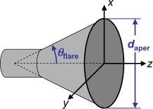
The aperture (horn mouth) sits in the XY plane of the antenna local coordinate system, with boresight along the +Z direction. The antenna is characterized by the following settings: Mouth Diameter, Flare Half-Angle, and Polarization.

The conical horn will not operate below the TE₁₁ cut-off frequency of a circular waveguide, given by f_cutoff> = (x'₁₁ c)/( π d_aper), where x'11 ~= 1.8412 is the first zero of the derivative of the first-order Bessel function of the first kind, c is the speed of light, and d_aper is the mouth (aperture) diameter. Attempts to simulate with a conical horn below this frequency will result in an error. Technically speaking, the cut-off frequency should be based on the smaller diameter of the waveguide, not the diameter of the horn mouth, and it should therefore be higher. However, since the waveguide diameter plays no other role in the conical horn model, it is left out of the specification parameters in the interest of simplicity, and we instead tie the cut-off frequency to the mouth diameter in this SBR+ parametric antenna model.

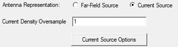
The dialog also lets you choose Antenna Representation as Far Field Source or as Current Source.

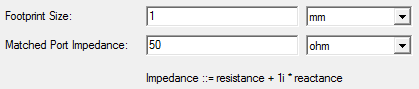
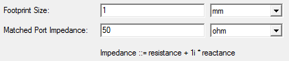
You specify parameters for mouth, flare half-angle, polarization, and matched port impedance.

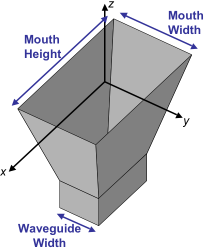
For conical horn antennas, the following figure explains the meaning of the dimensions.

If you select Current Source, the field for Current Density Over sample is enabled and the current source options button is enabled. For Current Source, you also need to specify Current Density Oversample, where the default value of 1.0 corresponds to 4 current-source samples per wavelength. Oversample values less than 1 are usually too course for an accurate result, while those greater than 2 usually do little to improve accuracy while harming run time. The default of 1.0 is the recommended setting for most cases, and we strongly discourage setting Current Density Oversample less than 1.0.

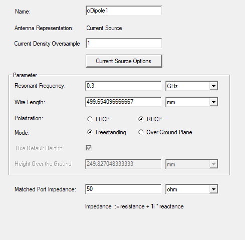
Cross Dipole

This antenna always uses a current source representation. Parameters are resonant frequency, wire length, polarization, and mode as free standing, or over ground plane. In the its Freestanding mode, the electric current sources represent two perpendicular arms of a dipole, one each along the Y and Z axes, driven with a 90 degree phase shift relative to each other to achieve the selected circular Polarization along the +X axis (it will be the opposite polarization along the -X axis). In its Over Ground Plane mode, the antenna arms are rotated to be parallel to the XY plane and at a default height along the Z axis of a quarter-wavelength at the specified Resonant Frequency. This allows the antenna to be placed directly on a metal surface of the SBR+ platform and have its reflected field constructively interfere with the direct incident field from the dipole arms when operating at the Resonant Frequency and in the +Z direction. You can switch off Use Default Height to manually set the height of the current source above the implied ground plane of this antenna if that better fits the design of the cross-dipole antenna to be simulated. You also specify matched port impedance.

Current Source Options opens a dialog with Use Global Setting (the default) or Specify, which enables the fields for Current Conformance, and Current Reduction settings to allow you to Thin Sources, and to specify a Power Fraction to Keep.

Current Source Options opens a dialog with Use Global Setting (the default) or Specify, which enables the fields for Current Conformance, and Current Reduction settings to allow you to Thin Sources, and to specify a Power Fraction to Keep.

Half-Wave Dipole

This antenna produces a far-field pattern of a center-fed thin dipole with a total length of a half-wavelength, with a peak Directivity of 2.15 dBi. The Half-Wave Dipole has no current-sources representation since it needs to be resonant at all simulation frequencies. For this reason, it is not recommended to locate it within two wavelengths of any SBR+ scattering geometry. If that is needed, one should instead consider to use the Wire Dipole or Horizontal Dipole in their current-sources representation.

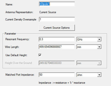
Horizontal Dipole

This antenna always uses a current-sources representation. It is intended for direct placement on a metal surface of the SBR+ platform given its built-in default height of a quater-wavelength.

Other parameters include current source options, resonant frequency, wire length, matched port impedance, and whether to use the default height or to override it and manually specify the height of the sources above the implied grounding surface. The default height is a quarter-wavelength at the specified Resonant Frequency. Assuming direct placement on a metal surface of the SBR+ platform, the intended context of this antenna, the reflected field from the platform will constructively re-enforce the direct field from the current sources in the +Z direction of the antenna.

Current Source Options opens a dialog with Use Global Setting (the default) or Specify, which enables the fields for Current Conformance, and Current Reduction settings to allow you to Thin Sources, and to specify a Power Fraction to Keep.

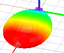
Parametric Beam

The Parametric Beam antenna for SBR+ produces an idealized pencil beam that can substitute as a simplification for a variety of aperture based antennas, including horns and broadside arrays. The main beam is pointed in the X direction of the antenna's local coordinate system and has the mathematical form, sin^Nvθ cos^Nhϕ , where Nv and Nh are internally determined according to the Vertical and Horizontal Beam Width settings, respectively. The antenna produces an idealized pencil beam (cosⁿθ) pattern) with user-defined beam widths and polarization. This antenna produces no side lobes or backlobes and only radiates in the forward half-space. The Parametric Beam antenna has no current-sources representation.

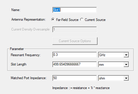
Parametric Slot

This antenna is based on an idealized sinusoidal (magnetic) current distribution for the slot along the X-axis of the coordinate system. The Far-Field pattern will vary according to the slot’s electrical length at the visualized frequency. When operated at the user-defined Resonant Frequency, the slot length is 0.5 wavelengths.

Note that changing the Resonant Frequency will update the Slot Length and vice versa.

The Parametric Slot is a ground-plane antenna whose intended placement is on a metal surface of the SBR+ scattering geometry or platform. In this context, use of the current-sources representation is strongly recommended. Although notionally located in the z = 0 plane of the antenna local coordinate system, the magnetic sources of the slot will instead be placed at a small offset height of λ/40 measured at the shortest wavelength of the simulation. This allows the parametric slot to be directly placed on a metal surface of the SBR+ platform without the need to manually offset it so that the sources don't inadvertently reside under the placement surface.

One can also select a far-field representation. However, given its assumed ground-plane context, the parametric slot radiates no far fields in its lower half-space, so all direct interaction with the placement platform is ignored during SBR+ simulation with this representation of the slot except for those surfaces of the platform or scattering environment that reside about the z = 0 plane of the slot antenna.

. The dialog also lets you choose Antenna Representation as Far Field Source or as Current Source.

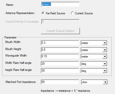
Pyramidal Horn

This frequency-dependent antenna approximates a flared rectangular horn with user-defined dimensions. It is based on the approximated field distribution of a rectangular cross-section pyramidal horn driven in the TE₁₀ waveguide mode. The model accounts for phase taper at the edges of the flat aperture (horn mouth) due to the elliptical phase front introduced by walls flaring from the rectangular waveguide feed at the throat of the horn.

The aperture (horn mouth) sits in the XY plane of the antenna local coordinate system, with boresight along the +Z direction. The antenna is characterized by the following geometric dimensions: Mouth Width, Mouth Height, Waveguide Width, Width Flare Half-Angle, and Height Flare Half-Angle. From these parameters, the waveguide height is implied. If the implied waveguide height is negative, an error report is generated with suggestions for adjusting the input dimensions to resolve the conflict.

The Pyramidal Horn will not operate below the TE₁₀ cut-off frequency of the rectangular waveguide, given by f_cutoff = c/2w, where w is the waveguide width and c is the speed of light. Attempts to do so will results in an error during simulation.

The dialog also lets you choose Antenna Representation as Far Field Source or as Current Source.

Current Source Options opens a dialog with Use Global Setting (the default) or Specify, which enables the fields for Current Conformance, and Current Reduction settings to allow you to Thin Sources, and to specify a Power Fraction to Keep.

Quarter-Wave Monopole

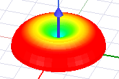
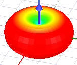
This antenna produces a far-field radiation pattern defined over a half-space (top half of a torus), consistent with an ideal quarter-wave monopole antenna over an infinite ground plane. It has a Directivity of 5.16 dBi in the upper half-space; no radiation gain in the lower half-space. This antenna only illuminates objects above the monopole and will not capture direct interactions with its placement surface on the SBR+ geometry. To model the interaction of a monopole with its supporting SBR+ platform, users should instead use the Wire Monpole in its current-sources representation.

Short Dipole

This antenna produces a far-field pattern of an ideal Hertzian(electrically short) electric dipole with a peak Directivity of 1.76 dBi. The Short Dipole is suitable as an idealized, yet still physical electromagnetic point source that stands off two or more wavelengths from any scattering geometry. It only has a far-field representation with no higher-order near-field terms. If the antenna is to be placed within one or two wavelengths of the SBR+ scattering geometry, one should consider to instead use the Wire Dipole or Horizontal Dipole in their current-sources representation since these have a valid near-field description.

Small Loop

This antenna produces a far-field pattern consistent of an ideal Hertzian loop (electrically short) magnetic dipole with a peak Directivity of 1.76 dBi. Because it only supports a far-field representation, it should only be used when it can be placed two or more wavelengths away from any SBR+ scattering geometry.

Wire Dipole

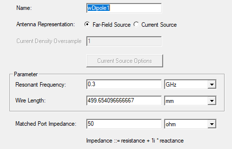
This antenna is based on an idealized sinusoidal current distribution of a wire dipole along the Z-axis of the antenna coordinate system. The Far-Field pattern will vary according to the dipole's electrical length at the visualized frequency. When operated at the user-defined Resonant Frequency, the wire is a half-wavelength long. Note that changing the Resonant Frequency will update the Wire Length and vice versa.

The Wire Dipole offers both a far-field and current-sources representation. The former is more computationally efficient to use in an SBR+ simulation, but the current-source representation should be used if the antenna is to be placed within 2 wavelengths of the SBR+ scattering geometry or its Wire Length is a significant fraction of its displacement from the scattering geometry.

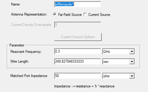
Wire Monopole

This antenna is based on an idealized sinusoidal current distribution for the monopole along the Z-axis of the antenna coordinate system. The Far-Field pattern will vary according to the monopole's electrical length at the visualized frequency. When operated at the user-defined Resonant Frequency, the monopole is a quarter-wavelength long. Note that changing the Resonant Frequency will update the Wire Length and vice versa.

The Wire Monopole is a ground-plane antenna whose intended placement is on a metal surface of the SBR+ scattering geometry or platform. In this context, use of the current-sources representation is strongly recommended.

One can also select a far-field representation. However, given its assumed ground-plane context, the Wire Monopole radiates no far fields in its lower half-space, so all direct interaction with the placement platform is ignored during SBR+ simulation with this representation of the monopole except for those surfaces of the platform or scattering environment that reside above the z = 0 plane of the monopole antenna.