Design Settings for HFSS

The HFSS>Design Settings command displays a dialog with tabs appropriate to the HFSS Solution settings. For HFSS driven solutions, using Modal or Terminal options, the tabs include Set Material Override, for automatic Lossy Dielectrics, DC Extrapolation, Validations, for S-Parameter definition, for Export On Completion, and for Adaptive Mesh.

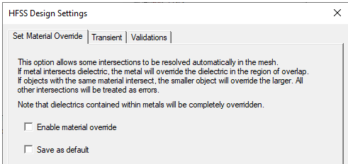
For Transient designs, the dialog contains Set Materials Override, Validations, and a Transient tab.

For SBR+ Designs,

For Eigenmode or Characteristic Mode, only the Set Materials Override and Validations tabs are needed..

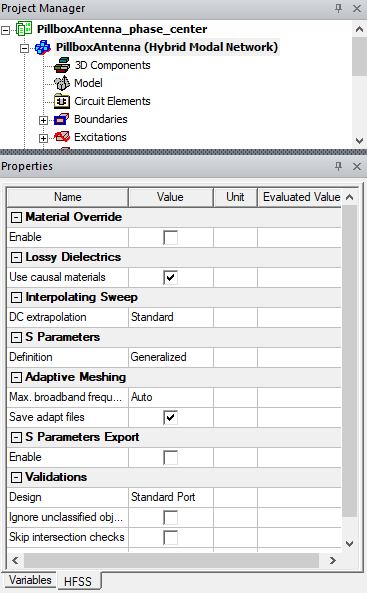
Selecting a current design in the Project tree also displays the Design Settings in Properties window under the solver tab.

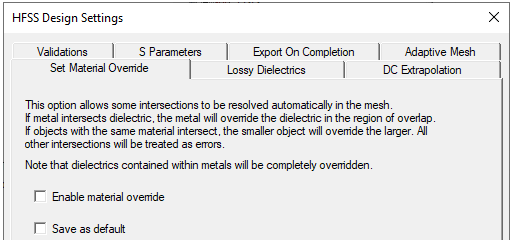
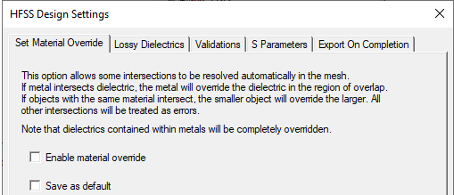
Set Material Override Tab

The Set Material Override tab includes text note and a check box to Allow metals to override dielectrics. The purpose of this feature is to allow you to avoid doing explicit subtraction in the modeler. One example application is a via that passes through many dielectric layers--with the option turned on, the via does not have to be subtracted from the layers.

The Set Material Override option allows some intersections to be resolved automatically in the mesh. If metal intersects dielectric, the metal overrides the dielectric in the overlap region. (That is, the metal object is subtracted from the dielectric.) If objects with the same material overlap, the small object overrides the larger. (That is, the small object is subtracted from the larger.) All other intersections are treated as errors. Normally, the modeler considers any intersection between 3D objects to be an error.

To use this feature, check Enable material override.

In the meshing process, the dielectrics are locally overwritten by the metals in the intersecting region. That is, the part of the dielectric that is inside the metal is removed, and if the dielectric is completely inside, the whole object disappears.

Lossy Dielectrics Tab

This option applies frequency dependent lossy materials for the solver and post processor. The materials are not modified in the design. Instead, the Djordjevic-Sarkar model is applied before the material is passed to the solver or used for post processing.

• Automatically use causal materials. (Default, unchecked).

If the assigned material is already frequency dependent, automatic creation of frequency dependent lossy materials is ignored.

This feature addresses cases where you only have simple constant material properties available, but want to automatically apply a general-purpose frequency dependence to ensure causal solutions when solving frequency sweeps. Automatic causal material calculations are not performed under the following circumstances:

• If the solution type is eigenmode
• If the material permittivity or loss tangent is anisotropic
• If the material permittivity or loss tangent is spatially dependent
• If the material permittivity or loss tangent is frequency dependent
• If the material itself is not a lossy dielectric

Otherwise, when enabled the Djordjevic-Sarkar model is applied to all constant lossy dielectrics. These are defined as having a constant permittivity that is greater than one and a constant loss tangent that is greater than zero. The inputs to the Djordjevic-Sarkar model are the material's constant permittivity and loss tangent, plus the standard default values of measurement frequency (1 GHz), DC conductivity (1e-12 S/m), and DC permittivity (none ). The outputs from the Djordjevic-Sarkar model are the expressions for permittivity and conductivity. These expressions, plus zero loss tangent, are used in place of the material's constant properties.

When reading legacy designs (HFSS 12 and earlier), this feature is unchecked.

DC Extrapolation Tab

The DC Extrapolation tab option affects Interpolation Sweep setup. If you select Standard DC Extrapolation, the software computes values automatically, and the tab for DC Extrapolation does not appear on the Interpolating Sweep setup.

For Advanced DC Extrapolation, the Interpolating Sweep setup includes the DC Extrapolation tab, so you can set a Minimum solved frequency.

The Design Settings dialog also contains check boxes to Save As Default.

Validations Tab

The Validation tab offers choices for Model validation and HFSS validations to control the extent of validations performed, and therefore the time involved.

Model Validation choices are whether to:

• Ignore unclassified objects
• Skip intersection checks

You also control the Entity check level as Strict, Basic, Warning Only, or None.

The HFSS choices are whether to:

• Perform full validations with standard port validations. Standard validation does not check for internal or floating ports.
• Perform full validations with extended port validations. The Extended validation checks to see if a wave port has been applied to an internal face, or if a wave or lumped port does not have solve inside geometry on either side.
• Perform minimal validations. This choice disables port validation options (neither is performed), and skips boundary overlap validation.

The default is to Perform Full Validations. However you can set your own default choices by using the Save as Default check box.

S Parameters Tab

The S Parameters tab offers choices for S parameter definition for post processing as Generalized or Power. Power S parameters are calculated for the reporter, S parameter export, and the Matrix display. Changing the setting between Generalized or Power updates reports and exported data, but not the solve status.

Generalized S parameters are based on the relationship between scattered and incident fields; hence, it is possible to have S parameters greater than one if there is a strong imaginary component of the reference impedance. While correct, some circuit designers may find this counter-intuitive and prefer instead to use Power S parameters. Power S parameters are based on the transfer and reflection of power, which must be less than unity for any passive device.

Note: Setting Power S using UpdateRegistry requires a workaround.

Adaptive Mesh Tab

Maximum Number of Frequencies for Broadband Adapt: Normally the decision for how many frequencies to use for broadband adaptive meshing is set automatically. Because the decision is not straightforward, this option is for advanced users to manually set the maximum number of frequencies to solve during broadband adaptive meshing. This feature works for both auto and advanced simulation setups.

Save Adaptive Mesh Control Files: Allows you to disable saving adaptive mesh control files to save disk space. However, if unchecked, reverting the mesh to a previous pass requires adapting from the initial mesh. Changing the setting reverts to the initial mesh.

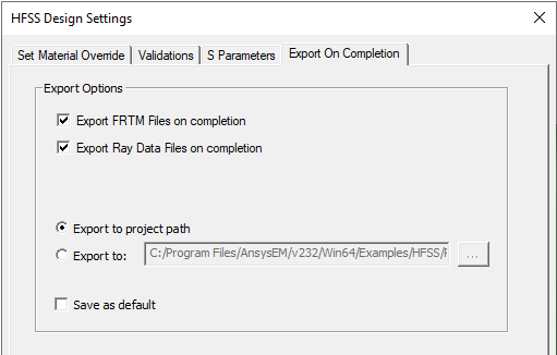
Export On Completion

This applies to HFSS 3D Driven Modal/Terminal and HFSS 3D Layout and, in a simpler way, to SBR+ or Hybrid solution type designs.

The SBR+ solver, when examining range-doppler problems, produces its raw data in a proprietary file format with the extension “.frtm”. The Export On Completion setting lets you specify that output, and enabled, lets you either export to the project path or a specified file location.

In addition, the SBR+ ray data export feature is available for Hybrid SBR+ and SBR+ solution-type, for any frequency domain definition (single point, discrete sweep, interpolating sweep, FFL, etc.), source and/or radiation domain configuration, in range-Doppler simulations, and for VRT plots, in a proprietary file format with the extension “.hdm”. The ray export feature also supports distributed simulations both in Hybrid and SBR+ solution-type. The solution distribution differs between Hybrid and SBR+ solution-type. In Hybrid, SBR+ distributes jobs according to frequency domain subsets of the original domain, but all distributed jobs shoot the same number of rays. In SBR+ solution-type, all distributed jobs share the same complete frequency domain, but each job only performs a subset of the ray tracing algorithm.

The simulation Ray Export settings appear under the Export On Completion tab in the HFSS Design Settings.

By default, the SBR+ files appear in a sub-folder along side the aedtresults folder, and is named .aedtexport. Within that folder, exported files are segregated by design name, setup name, parametric variation, and date/time of solve.

It is your responsibility to ensure that there is enough available space on disk to perform ray export both for solver and VRT. The ray export algorithm performs very limited disk-space availability checks.

If you name a specific folder, all exports (named distinctly) are placed in that folder.

A frequency group represents a subset of frequencies chosen from the frequency domain of the simulation. In Hybrid SBR+, each group simulates up to N frequencies, with N the number of tasks allowed for each distributed simulation. In SBR+ solution-type, all frequencies are simulated at once (e.g., all files are under Group_0), but each node only processes a subset of the total number of rays. There is currently no way of knowing what frequencies belong to what group other than partially parsing one of the files in the export directory.

Ray Export files are exported either under a default <project_name>.aedtexports folder, or in a folder of the users choice. Exports are grouped by export date and time, and then by design, solution/variation type, and lastly by group number. A group represents a subset of frequencies chosen from the frequency domain of the simulation. In Hybrid SBR+, each group simulates up to N frequencies, with N the number of tasks allowed for each distributed simulation. In SBR+ solution-type, all frequencies are simulated at once (e.g., all files are under Group_0), but each node only processes a subset of the total number of rays. There’s currently no way of knowing what frequencies belong to what group other than partially parsing one of the files in the export directory.

Ray export file names follow a specific format:

(sbr|cw)export_src<srcName>_rank<rankNumber>_b<batchNumber>.hdm

The export type (sbr|cw) indicates if the .hdm contains SBR/UTD or CW ray exports. srcName follows the following convention:

FEBI or NF/FF links: _<excitation>_<port/mode>

parametric antennas or FFD/NFD files: _<excitation>

bistatic plane-wave: integer index <N> starting at 0, incidence angle

monostatic plane-wave: 0

The other two file-name groups are simply numerical identifiers to disambiguate ray exports.

The .hdm format begins with an ASCII header that completely describes the file format and content in both a human-readable way and a machine-readable way. Parsers for the hdm format are available in the pyAEDT package. A binary section follows the ASCII header. Please refer to the available parsers and to a hdm header for more information.

For HFSS driven solutions, or HFSS 3D Layout, after a sweep (discrete, interpolating, or fast) simulation is successfully completed, you can choose to automatically save a Touchstone file for the sweep’s S-parameter data into a folder. By default, this folder is named after the project. The exported directories/files are not managed by Ansys Electronics Desktop. That is, you can rename the project, design, setup, etc. and previously exported directories/files will NOT be renamed. For Optimetrics simulation, export is per solved variation. Touchstone files are exported only when the simulation completes without error

The Export S Parameters tab lets you Set/View Export Preferences and specify whether to Export Touchstone file after completing frequency sweep. Checking the export feature enables you choose to override the default project path. You can save your preferences as the default. Preference is per design type and per user. This means that the same user can have one set of preferences for 3D layout design and another set for HFSS 3D design.

Clicking the Set/View Export Preferences button opens the SYZ Data Export Options dialog.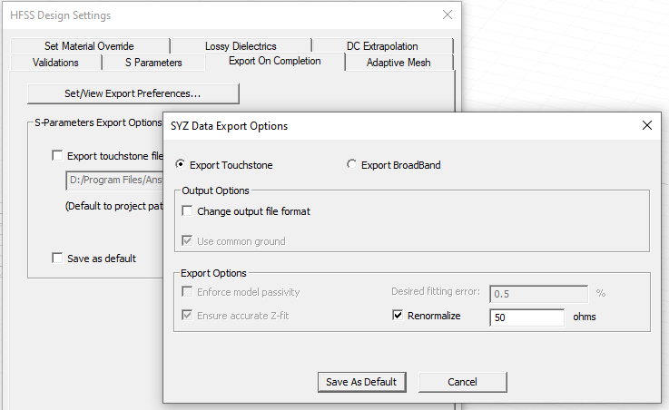

The SYZ Data Export Options dialog contains a range of choices for Output format, including advanced options.

Macromodel Output Options.

Checking Change output file format displays additional choices that lets you select Touchstone 1.0 or Touchstone 2.0, as well as additional Touchstone options. Unchecking conceals the output file format choices.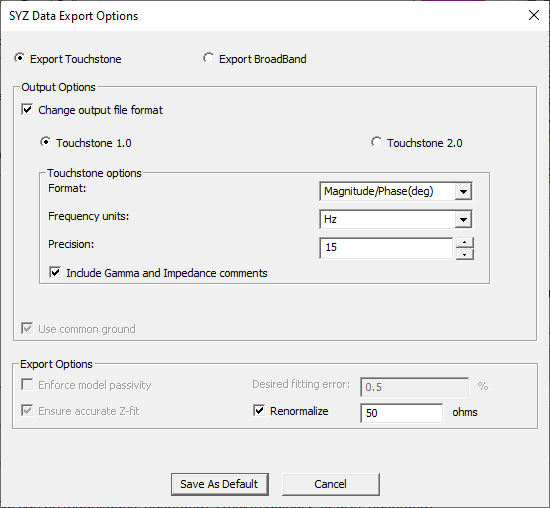

• Format can be Magnitude/Phase(deg), Real/Imaginary, or dB/Phase(deg)
• Frequency units can be Hz, KHz, MHz, or GHz.
• Precision can be to the number of digits you specify.
• Include Gamma and Impedance comments. Unchecking allows you to suppress writing Gamma and Impedance.

You can also specify whether to Use common ground.

Macromodel Generator Options include:

• Enforce model passivity
• Desired fitting error percent
• Ensure accurate Z-fit
• Renormalize to a specified value
  

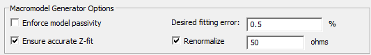
Clicking the Advanced option button displays or hides the Advanced options.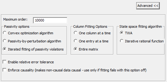

Choosing Save As Default saves the selected options as your user preferences for automatic Touchstone export and for subsequent launch of the SYZ Data Export options.

Automatic Touchstone File Exports

The top level export folder is named after the project file.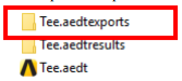

Within the top level export folder, a separate folder is created for each design that has exported touchstone files.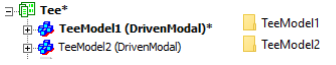

In each design export folder, exported files are further organized based on the setup that is being simulated. For non-Optimetrics simulation, the sub-folder is named after the solve setup and followed by a “time-stamp” string2. For Optimetrics simulation, the sub-folder is named after the Optimetrics setup and followed by a “time-stamp”. string.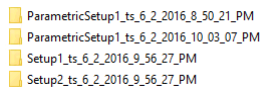

Touchstone files are exported into these sub-folders and an index file is created per sub-folder to help users track the exported data. For non-Optimetrics export, files are named as <Sweep>_DV<unique ID>.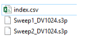

For Optimetrics export, files are named as <Setup>_<Sweep>_DV<unique ID>.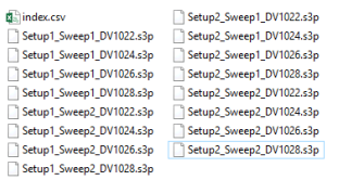

The index.csv can be opened in Excel. Variation information is listed in row/column format for readability.