Visual Ray Trace (VRT) for SBR+ Simulation

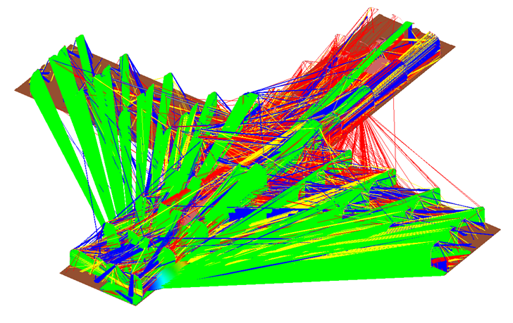
Visual Ray Trace (VRT) is a powerful feature available in HFSS for visualizing the ray geometry and interactions for an SBR+ simulation. Since SBR+ relies on “painting” physical optics (PO) currents on the geometry, VRT can provide valuable insight for analyzing these PO contributions from the direct illumination first-bounce rays and the multi-bounce rays we propagate using geometric optics (GO). The “hit point” locations for each ray bounce may be visualized, the ray paths between each bounce may be visualized, and the “footprints” that are used to integrate the PO currents at each bounce may be visualized. The VRT feature includes a number of other rendering controls and options to filter whole ray tracks or individual ray bounces, visualize ray scattering directions, and color ray point/lines/footprints according to different criteria. The VRT feature also lets you use SBR+ with PTD and UTD to account for additional phenomenology. You can now create SBR VRT plots with blockages, as described in Create VRT (Visual Ray Trace) Plot with Geometry Blockage

Prerequisites

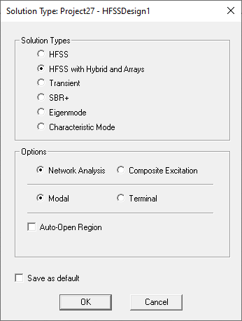
To use the VRT feature, you must have an HFSS design with either the SBR+ solution type or with the HFSS with Hybrid and Arrays solution type and one or more SBR+ hybrid regions. Various boundary conditions (BCs) and material properties may be assigned to the SBR+ geometry, as detailed in Geometry, Boundaries and Dielectric Region Support in SBR+. Use of any unsupported boundaries or material configurations will produce an error if attempted with VRT. Note that for all Layered Impedance boundaries assigned to an SBR+ region geometry the surface roughness must be set to “0”.

Using Visual Ray Trace (VRT) in Ansys Electronics Desktop

1. Once you have an appropriate HFSS design, there are three different ways in the user interface to create a new Visual Ray Trace Plot:

• Right-click the Field Overlays icon in the Project Tree and select Plot VRT... from the short cut menu.
• Right-click the 3D Modeler window and select Plot VRT... from the pop-up menu.
• Click HFSS>Fields>Plot VRT...

After you use one of these approaches, the Create VRT Plot dialog displays:

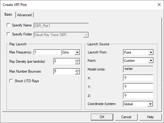
To Specify Name check the box to enable the text field. To Specify Folder, check the box to enable the selection menu.

2. Set the Ray Launch Parameters

• VRT plots do not have to be configured the same as your HFSS design/analysis setup. You can use VRT to experiment and plot rays with different types/locations of ray sources independent of your full HFSS simulation run.
• Max Frequency and Ray Density parameters control the density of rays that will be launched from the source for the Visual Ray Trace.
• Launch From parameters configure the source ray launch setup for the VRT rays. You can use a custom specified XYZ coordinate, an existing Point object, a Plane-Wave incident direction specified in Theta/Phi, or from an Antenna 3D Component. More detailed information/instructions about using Antennas with VRT can be found under Parametric Antennas and Parametric Array Antennas for VRT Plots. By default, the Launch From selection is Point and launched from the global coordinate system origin.
  Note: In the case of a FE-BI Hybrid Region, by design the VRT rays launch from the center of the FE-BI, rather than a port location in the FE-BI portion of the design. For example, in the following image, the highlighted box is assigned as a FE-BI Hybrid Region, and the center of the box becomes the VRT launch point rather than the antenna within the Hybrid region.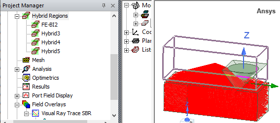
  
• Shoot UTD Rays controls whether the plot generates additional UTD rays that represent diffraction within the Keller cone off the edge to generate rays in the shadow region. If you modify the SBR+ initial mesh and/or wedge settings, the VRT plot with UTDs rays may need to be invalidated since it depends on both. See the discussion of SBR+ Wedge settings.

3. Optionally, select the Advanced tab. Here you can specify a Filter for “Shoot Filter” to limit the number of rays generated. You can select from these to diagnose model issues or to explore sub-regions of a very large or dense mesh:

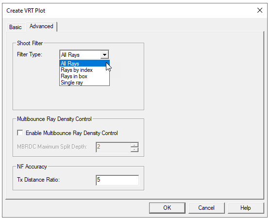
• All Rays (normal, default behavior)
• Rays by index: ray indices may be used to limit the rays to a specified range/interval by Start/Stop, or can skip rays by changing the Step value from 1
• Rays in box: a Box (model or non-model) can be created or selected from the model in the area near the VRT launch point. The Box filters generation of rays whose first bounce is in the area of the SBR+ region geometry defined by the Box extents. A valid Box can be defined using either a Global/Relative coordinate system, but it cannot have additional geometry operations (Rotate, Move).
• Single Ray: specify a theta/phi angle relative to the launch point for a single ray to be generated

4. The Advanced tab also allows you to Enable Multibounce Ray Density Control.
   
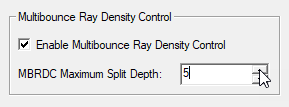
   Use the checkbox to Enable Multibounce Ray Density Control and enter the maximum number of subdivisions to be used in the plot. Enabling the feature may increase the solve time. The MBRDC Maximum Split Depth field value increases the number of spawned ray tracks on each ray bounce. The MBRDC algorithm is designed to achieve the ray density per wavelength criterion at any bounce depth. If a footprint at depth N in a ray track does not satisfy the ray-density criterion, the MBRDC algorithm attempts a refined ray shoot from an earlier bounce, just for the ray in question. The size of the triggering footprint informs the level of refinement. If the refined shoot is not successful in achieving the desired footprint size, or new footprints are too large, the MBRDC algorithm attempts further, recursive refinements. The MBRDC Maximum Split Depth setting limits how aggressively the refinement algorithm is applied by specifying the maximum number of split recursions. For this reason, linear increases in MDRC Maximum Split Depth can yield a geometric progression in the total number of rays shot and associated solution time.
   
   When both MBRDC and UTD are enabled, first-bounce UTD rays and bright points on wedges are recomputed during the MBRDC splitting process, but only the original raytrack is rendered up to the 1st bounce. Similarly, length-based ray filters are applied to the original UTD initial ray track up to 1st bounce rather than using the information in the additional MBRDC tracks. This is a known limitation.
   
5. The Advanced tab allows you to specify a Tx Distance Ratio to oversample footprints near the ray source. Fields change rapidly near the Tx antenna. When you place a Tx antenna near a surface, HFSS SBR+ adaptively increases the ray density above the normal level, but only for the nearby surfaces. This ensures adequate sampling of the Tx radiation field by the rays. For close-proximity surfaces, HFSS SBR+ further subdivides these sub-surfaces to maintain a minimum ratio between distance-from-Tx-to-surface and maximum-linear-dimension-of-surface. By default, this ratio threshold is set to 5. Normally, this setting is adequate. To increase the over-sampling, increase this ratio setting above 5. To switch off the over-sampling feature, set this ratio very low, say 0.01. Even when set very low, HFSS SBR+ will still shoot rays at a minimum density according to the Ray Density parameter
6. Click Done to dismiss the dialog to run the VRT generation to produce SBR+ ray data. Only the geometries contained in the SBR+ regions are used for the VRT ray generation.

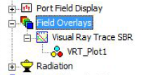
A new “Visual Ray Trace SBR” plot folder is created under Field Overlays, which contains one or more “VRT_Plot” items.

You can right-click on the VRT plot to display the Export Plot... command.

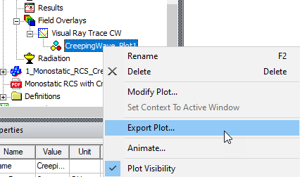
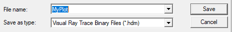
This allows you to export Visual Ray Trace Binary Files using a .hdm suffix.

If you run Plot VRT... again, that creates an additional VRT plot item under the “Visual Ray Trace SBR” folder, or a different folder name if you specify one in the Create VRT Plot dialog.

Create VRT (Visual Ray Trace) Plot with Geometry Blockage

Ppreviously Visual Ray Trace (VRT) plots did not support use of "Model Blockage” geometry - that geometry is not considered as part of the VRT geometry since it is not part of the SBR+ region. We added VRT support for this antenna blockage geometry in the same way that it is now included for the SBR+ simulation. Any geometry objects in the SBR+ region identified as “Model Blockage” will be ignored on the first bounce and included on any multi-bounce for VRT when the associated source antenna is used as the VRT source.

1. Create/open an design with HFSS with Hybrid and Arrays solution type.
   
   
2. Configure an HFSS design with SBR+ antenna blockage for either SBR+ or HFSS with Hybrid and Arrays solution type.
   
3. To create a new VRT plot select the menu option Field Overlays > Plot VRT> SBR to open the Create SBR VRT Plot dialog.
4. Change the Launch From: setting to “Antenna” and select the desired Antenna/Port from the available hybrid Antenna/Port source/excitation regions.
   
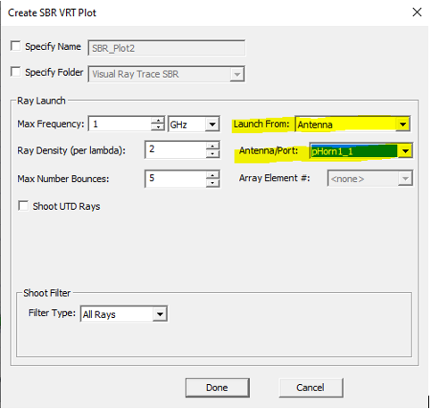
5. Click Done to create the plot with SBR rays, which will include the configured behavior of any SBR+ antenna blockage geometry.

VRT Plot Properties

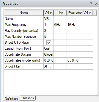
The Properties of each VRT_Plotn item are the same as those created in the Create VRT Plot dialog.

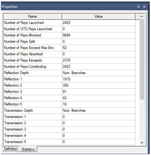
Each Visual Ray Trace SBR plot has an additional read-only tabbed property page that displays Ray Statistics output from the ray generation process.

Modifying VRT Plots

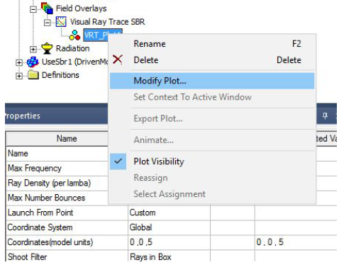
You can modify VRT Plot node properties directly in the Properties window to cause immediate updates to the plot data. You can also right-click the plot item and select Modify Plot… to again bring up the Create VRT Plot dialog to make multiple changes and then commit them to the same, or a differently named plot.

Design Edits that Invalidate the Mesh Invalidate VRT Plots

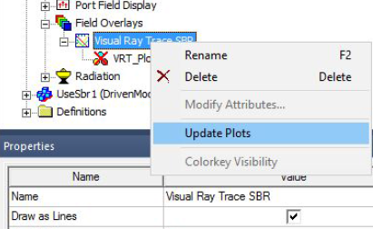
Any design edits that invalidate the mesh (geometry delete, modify, or change in boundary condition assignment) also invalidates VRT plots. HFSS does not automatically regenerate the VRT plot after a design edit. You can update plots update by right-clicking on the Visual Ray Trace SBR folder and selecting Update Plots or by double-clicking on the VRT plot item in the Project Manager, which will either be invalidated with a red ‘X’ or greyed out if it needs manual update.

Modification in SBR+ Wedge Setting parameters invalidates the VRT plot when “Shoot UTD Rays” is turned on.

In addition for UTD rays, a modification to the geometry and/or boundary conditions should automatically cause new SBR+ wedge to be generated whenever the VRT plot is manually updated.

Visual Ray Trace SBR Folder Properties

All the render and filter parameters appear as Properties of the parent Visual Ray Trace SBR folder. Each “Visual Ray Trace SBR” plot folder provides a grouping of render/filter attributes. Much like setting specific plot attributes like 2D plot extents, scaling, colormaps, etc., the render and filter parameters for all VRT plots are performed at this folder level. The different categories of render and filter operations are kept as separate tabs for: Rendering, Filters, and Rx Filters.

All render and filter property changes are immediate and will automatically refresh the 3D modeler window

Rendering Properties Tab

The Rendering tab properties control which items are drawn for each ray track:

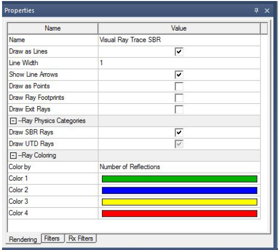
• Draw as Lines: show the “rays” connecting the launch point, each intersection point, and the exit point.
• Draw as Points: show the point for each ray bounce where we intersect the geometry.
• Draw Ray Footprints: show the ray tube projection for each ray bounce.
• Draw Exit Rays: show the final ray of a ray track if/when it exits the geometry and is scattered away (note: ray tracks that reach “Max Bounce” may not have an exit ray).
• Draw SBR Rays: toggles SBR rays on and off.
• Dray UTD Rays: toggles UTD rays on and off.

Ray Coloring controls:

• Color by: Number of Reflections: the full ray track branch (from creation to exit) is colored according to the number of reflection bounces occurring for that ray track segment.
• Color by: Number of Transmissions: the full ray track branch (from creation to exit) is colored according to the number of transmission bounces occurring for that ray track segment.
• Color by: Bounce Number: each ray bounce of the ray track branch is colored a different color, according to the bounce number of that ray

Filters Properties Tab

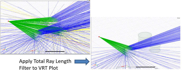
The Filters properties tab controls which ray tracks and/or bounces are shown in the 3D modeler window. For example, you could generate a VRT plot and apply a filter.

Intially, the checkboxes for Full Ray Tracks and Filter Individual Ray Bounces are unchecked. Your selections for each type of control enables additional fields for specifying exactly how and what to filter for Full Ray Tracks and/or Individual Ray Bounces.

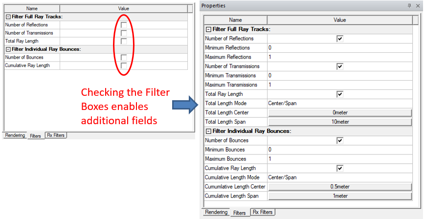
• Filter Full Ray Tracks:
• Number of Reflections: use the Minimum and Maximum Reflections values to show only those ray tracks within the specified range of reflected bounces (filters out whole ray tracks).
• Number of Transmissions: use the Minimum and Maximum Transmissions values to show only those ray tracks within the specified range of transmitted bounces (filters out whole ray tracks).
• Total Ray Length: use Total Length Mode of either Center/Span or Min/Max. You can assign length values as a variable. Using a variable permits you to creating an animation by sweeping the variable.
  
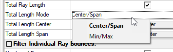
  Selecting Center/Span enables buttons for Total Length Center and Total Length Span. Clicking one of these buttons opens Slider window that allows you to modify the filter values and see in real-time the changing rays in the model view window.
  
  
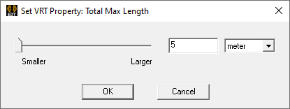
  Selecting Min/Max enables buttons for Total Min Length and Total Max Length. Clicking a button opens a Slider window for real time control of the modeler window.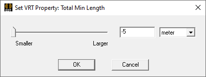
  
  
  
  
• Filter Individual Ray Bounces:
• Number of Bounces: use the Minimum and Maximum values to show specific bounce numbers from all ray tracks (filters out individual bounces).
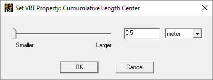
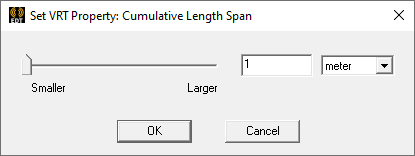
• Cumulative Ray Length: use with the Center/Span or Min/Max selections. You can assign length variables as the value. Using a variable allows you to animate the plot by sweeping that variable. Selecting Center/Span enables buttons for Cumulative Length Center and Cumulative Length Span. Clicking one of these buttons opens Slider window that allows you to modify the filter values and see in real-time the changing rays in the model view window.
  
  
  Selecting Min/Max enables buttons for Cumulative Length Center and Cumulative Length Span. Clicking a button opens a Slider window for real time control of the modeler window.
  
  
  

Note these Filters can be used in combination to show only the specified ray bounces from a filtered set of ray tracks (e.g., show only the 2nd and higher bounces for ray tracks that have no transmitted rays).

Rx Filter Properties Tab

Use an “Rx Filter” to show only ray tracks that satisfy a specified scatter direction (far-field) or spatial filter (near-field).

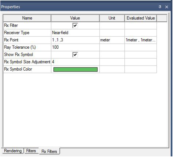
• Receiver Type: Near-field: use a spatial probe type of filter to only show ray tracks that go near a specified point/location, within some tolerance
• Receiver Type: Far-field: use a far-field directional filter to only show ray tracks whose exit ray direction (scattering direction) is the specified theta/phi angle, within some tolerance

SBR+ with PTD and UTD

For SBR+ simulations, the Physical Theory of Diffraction (PTD) and Uniform Theory of Diffraction (UTD) features can account for additional phenomenology not well predicted by plain SBR due to truncation of Physical Optics (PO) currents at sharp angular discontinuities (“wedges”) on metallic surfaces. PTD is a numeric correction to the results, while UTD is a method to generate additional rays that represent diffraction within the Keller cone off the edge to generate rays in the shadow region. To use these features for the SBR+ solver and Visual Ray Trace (VRT) in the desktop UI, we provide you with a way to specify the location of these “wedges” on the 3D geometry model, so that their contributions for PTD and UTD may be determined when these features are enabled. Typically, there may be thousands of candidate edges on a triangular mesh model, and many hundreds or thousands of “wedges” to include for the simulation. You often need some additional guidance in determining which wedges to include in the simulation, and you may want to specify areas of the model include or exclude wedges in the analysis. You can provide an angular criteria can for the minimum exterior wedge angle to help filter the desired set of wedges, and you can choose to include or exclude wedges from “knife edges”, or open (non-shared) edges from a geometry such as a very thin flat plate. You can view the set of wedges to be used for the SBR+ or VRT simulation in the 3D modeler window, and subsequently regenerate the set of wedges if necessary with different criteria.

Scenarios for using VRT toVisualize UTD Rays include the following:

• Setup an SBR+ simulation with PTD/UTD and check the UTD rays before solving. Set the launching point for a VRT plot to a location where an antenna will be used. Open the statistics tab, and check the Number of UTD rays launched. If the value is greater than 0, then the simulation will benefit from the SBR+ PTD/UTD feature.
• Explore an antenna placement for possible UTD rays. To do this, create variables that control where the antenna will be placed. Apply that variable to a relative coordinate system and/or a point. You can then create a VRT plot where the launching point uses the relative coordinate system or point you have defined. Enable the Shoot UTD rays feature and make those rays visible. After drawing the plot, animate it, and set the swept variable as one that controls the coordinate system or point placement. You can then observe the UTD rays drawn and tune the antenna placement based on the existence of UTD rays.