


Hybrid initialization is yet another initialization method in Ansys Fluent. The other initialization methods are standard initialization and FMG initialization. Hybrid initialization is a collection of recipes and boundary interpolation methods. It solves Laplace's equation to determine the velocity and pressure fields. All other variables, such as temperature, turbulence, species fractions, and volume fractions, will be automatically patched based on domain averaged values or a particular interpolation recipe.
For more information about hybrid initialization, see Hybrid Initialization in the Theory Guide.
For additional information, see the following sections:
The default initialization method for single phase steady-state flows is the Hybrid Initialization method.
Note: For other flow types, such as multiphase or unsteady simulations, the default initialization method is the Standard Initialization method. However both initialization methods are available for use in all flow conditions and types.
To use Hybrid Initialization, go to the Solution Initialization Task Page (Figure 36.17: The Solution Initialization Task Page for Hybrid Initialization) where you will select Hybrid Initialization.
![]() Solution →
Solution → ![]() Initialization
Initialization
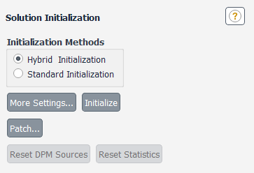
Note: In most cases, you need not do anything more than click the button. However, should you decide to modify the default settings for the hybrid initialization method, click .
If you click , the Hybrid Initialization dialog box (Figure 36.18: The Hybrid Initialization Dialog Box) will open. A host of settings that control the Hybrid Initialization strategy will be available for you to adjust.
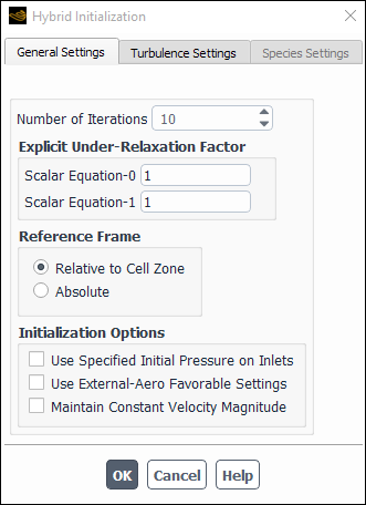
You can make adjustments in three different areas:
General Settings tab:
Number of Iterations uses a default value of 10. This is the number of iterations that will be performed while solving the Laplace equations to initialize the velocity and pressure. In general, you do not need to change the number of iterations. However, for complex and highly curved geometries, if the default number of iterations is not enough to reach the convergence tolerance of 1e-06 and the flow fields are not to your liking, then you may want to increase the number of iterations and re-initialize the flow.
Explicit Under-Relaxation Factor uses a default value of 1. This value will be used while solving the Laplace equation to initialize the velocity and pressure. In general, you do not need to change the explicit under-relaxation factor. However, for some cases, where the scalar residuals are oscillating and showing difficulty reaching the convergence tolerance of 1e-06, you may want to re-initialize the flow by reducing the under-relaxation factor. You may also want to increase the number of iterations to produce a smooth initialization field for the velocity and pressure.
Reference Frame is set to Relative to Cell Zone by default. If your problem involves moving reference frames or sliding meshes, indicate whether the initial velocities are absolute velocities or velocities relative to the motion of each cell zone by selecting Absolute or Relative to Cell Zone. If no zone motion occurs in the problem, the two options are equivalent. If the solution in most of your domain is rotating, using the relative option may be better than using the absolute option.
Initialization Options allows you to include the following options:
Use Specified Initial Pressure on Inlets if you want the specified pressure for Supersonic/Initialization Gauge Pressure at the inlet boundaries to be used for solving the Laplace equation for the pressure. Otherwise, Ansys Fluent uses a predetermined recipe to determine the initial pressure field, as described in Hybrid Initialization of the Theory Guide.
Use External-Aero Favorable Settings if you want to have the velocity potential patched with a linear value to help accelerate convergence of Scalar Equation–0 and to obtain a better guess of the velocity field for external-aero problems, such as flow over wings, airfoils, or automobiles.
Maintain Constant Velocity Magnitude if you want to use the flow direction obtained from solving the velocity potential (Scalar Equation–0), while maintaining a constant velocity magnitude throughout the computational domain. This option is helpful in some incompressible external flow problems, porous media problems, or if there are narrow channels where large undesirable velocities can be reached.
Turbulence Settings tab uses by default the domain averaged values for the turbulence parameters. If you want to use variable turbulence parameters you can deselect the Average Turbulent Parameters check box. When this option is disabled, then it calculates the turbulent parameters, such as kinetic energy and dissipation energy, using local flow parameters.
Species Settings tab will by default initialize secondary species with zero mass or mole fractions. If you want to specify the appropriate value for the species, you will need to enable Specify Species Parameters. Note that only the boundary species that you have selected in the Select Boundary Species dialog box appear in the list (see Figure 19.3: The Select Boundary Species Dialog Box). You can add or remove a species using the Select Boundary Species that can be accessed by clicking in the Solution Initialization task page.
In general, you do not need to make any extra adjustments to the hybrid initialization default settings. However, if the hybrid initialization is not producing the initial field to your liking, then you can play with the various options available in the Hybrid Initialization dialog box (described in Steps in Using Hybrid Initialization), or you can also use the patching option in addition to the Hybrid Initialization. For example, if you are solving a user-defined scalar, then hybrid initialization will initialize them with a value of zero. However, you can specify the value with which you want to patch.
Note: You can also use a user-defined function to initialize the flow or certain flow variable in conjunction with hybrid initialization.
Standard Initialization is the recommended initialization method for porous media simulations. The default Hybrid initialization method does not account for the porous media properties, and depending on boundary conditions, may produce an unrealistic initial velocity field. For porous media simulations, the Hybrid initialization method can only be used with the Maintain Constant Velocity Magnitude option.