


Rate-independent plasticity is characterized by the irreversible straining that occurs in a material once a certain level of stress is reached. The plastic strains are assumed to develop instantaneously (that is, independent of time). Several options are available to characterize different types of material behaviors:
Material Behavior Option
Bilinear Isotropic Hardening
Multilinear Isotropic Hardening
Nonlinear Isotropic Hardening
Classical Bilinear Kinematic Hardening
Multilinear Kinematic Hardening
Nonlinear Kinematic Hardening
Anisotropic
Extended Drucker-Prager
Extended Drucker-Prager Cap
Cast Iron
User-specified behavior (described in User Routines and Non-Standard Uses)
Except for user-specified behavior (TB,USER), each material-behavior option is described in greater detail later in this chapter. Figure 4.1: Stress-Strain Behavior of Each of the Plasticity Options represents the stress-strain behavior of each of the options.
Plasticity theory provides a mathematical relationship that characterizes the elastoplastic response of materials. There are three ingredients in the rate-independent plasticity theory: the yield criterion, flow rule and the hardening rule. Table 4.1: Notation summarizes the notation used in the remainder of this chapter.
The yield criterion determines the stress level at which yielding is
initiated. For multi-component stresses, this is represented as a
function of the individual components,  , which can be interpreted as an equivalent stress
 :
:
 | (4–4) |
where:
 = stress vector = stress vector |
Table 4.1: Notation
| Variable | Definition | Mechanical APDL Output Label |
|---|---|---|
 | elastic strains | EPEL |
 | plastic strains | EPPL |
 | trial strain | |

| equivalent plastic strain | EPEQ |
 | stresses | S |
 | equivalent stress | |
 | material yield parameter | |
 | mean or hydrostatic stress | HPRES |

| equivalent stress parameter | SEPL |
 | plastic multiplier | |
 | yield surface translation | |
 | plastic work | |
 | translation multiplier | |
 | stress-strain matrix | |
 | tangent modulus | |
 | yield criterion | |
 | stress ratio | SRAT |
 | plastic potential | |
 | deviatoric stress |
When the equivalent stress is equal to a material yield parameter σy,
 | (4–5) |
the material will develop plastic strains. If  is less than
  , the material is elastic and the stresses will
develop according to the elastic stress-strain relations. Note that
the equivalent stress can never exceed the material yield since in
this case plastic strains would develop instantaneously, thereby
reducing the stress to the material yield. Equation 4–5 can be plotted in stress space as
shown in Figure 4.2: Various Yield Surfaces for some of the plasticity
options. The surfaces in Figure 4.2: Various Yield Surfaces are known as
the yield surfaces and any stress state inside the surface is
elastic, that is, they do not cause plastic strains.
, the material is elastic and the stresses will
develop according to the elastic stress-strain relations. Note that
the equivalent stress can never exceed the material yield since in
this case plastic strains would develop instantaneously, thereby
reducing the stress to the material yield. Equation 4–5 can be plotted in stress space as
shown in Figure 4.2: Various Yield Surfaces for some of the plasticity
options. The surfaces in Figure 4.2: Various Yield Surfaces are known as
the yield surfaces and any stress state inside the surface is
elastic, that is, they do not cause plastic strains.


The flow rule determines the direction of plastic straining and is given as:
 | (4–6) |
where:
 = plastic multiplier (which determines the
amount of plastic straining) = plastic multiplier (which determines the
amount of plastic straining) |
 = function of stress termed the plastic
potential (which determines the direction of plastic
straining) = function of stress termed the plastic
potential (which determines the direction of plastic
straining) |
If  is the yield function (as is normally assumed),
the flow rule is termed associative and the plastic strains occur in
a direction normal to the yield surface.
is the yield function (as is normally assumed),
the flow rule is termed associative and the plastic strains occur in
a direction normal to the yield surface.
The hardening rule describes the changing of the yield surface with progressive yielding, so that the conditions (stress states) for subsequent yielding can be established. Two hardening rules are available: work (or isotropic) hardening and kinematic hardening. In work hardening, the yield surface remains centered about its initial center line and expands in size as the plastic strains develop. For materials with isotropic plastic behavior this is termed isotropic hardening and is shown in Figure 4.3: Types of Hardening Rules (a). Kinematic hardening assumes that the yield surface remains constant in size and the surface translates in stress space with progressive yielding, as shown in Figure 4.3: Types of Hardening Rules (b).
The yield criterion, flow rule and hardening rule for each option are summarized in Table 4.2: Summary of Plasticity Options and are discussed in detail later in this chapter.

Table 4.2: Summary of Plasticity Options
| Name | TB Lab | Yield Criterion | Flow Rule | Hardening Rule | Material Response |
|---|---|---|---|---|---|
| Bilinear Isotropic Hardening | PLASTIC
(TBOPT = BISO) | von Mises/Hill | associative | work hardening | bilinear |
| Nonlinear Isotropic Hardening | NLISO | von Mises/Hill | associative | work hardening | nonlinear |
| Classical Bilinear Kinematic Hardening | PLASTIC
(TBOPT = BKIN) | von Mises/Hill | associative (Prandtl-Reuss equations) | kinematic hardening | bilinear |
| Nonlinear Kinematic Hardening | CHAB | von Mises/Hill | associative | kinematic hardening | nonlinear |
| Extended Drucker-Prager | EDP | von Mises with dependence on hydrostatic stress | associative or non-associative | work hardening | multilinear |
| Cast Iron | CAST | von Mises with dependence on hydrostatic stress | non-associative | work hardening | multilinear |
| Gurson | GURS | von Mises with dependence pressure and porosity | associative | work hardening | multilinear |
If the equivalent stress calculated using elastic properties exceeds the material yield, then plastic straining must occur. Plastic strains reduce the stress state so that it satisfies the yield criterion, Equation 4–5. Based on the theory presented in the previous section, the plastic strain increment is readily calculated.
The hardening rule states that the yield criterion changes with work hardening and/or with kinematic hardening. Incorporating these dependencies into Equation 4–5, and recasting it into the following form:
 | (4–7) |
where:
 = plastic work = plastic work |
 = translation of yield surface = translation of yield surface |
 and
and  are termed internal or state variables.
Specifically, the plastic work is the sum of the plastic work done
over the history of loading:
are termed internal or state variables.
Specifically, the plastic work is the sum of the plastic work done
over the history of loading:
 | (4–8) |
where:

and translation (or shift) of the yield surface is also history dependent and is given as:
 | (4–9) |
where:
 = material parameter = material parameter |
 = backstress (location of the center of
the yield surface) = backstress (location of the center of
the yield surface) |
Equation 4–7 can be differentiated so that the consistency condition is:
 | (4–10) |
Noting from Equation 4–8 that
 | (4–11) |
and from Equation 4–9 that
 | (4–12) |
Equation 4–10 becomes
 | (4–13) |
The stress increment can be calculated via the elastic stress-strain relations
 | (4–14) |
where:
 = stress-strain matrix = stress-strain matrix |
with
 | (4–15) |
since the total strain increment can be divided into an elastic and plastic part. Substituting Equation 4–6 into Equation 4–13 and Equation 4–15 and combining Equation 4–13, Equation 4–14, and Equation 4–15 yields
 | (4–16) |
The size of the plastic strain increment is therefore related to the total increment in strain, the current stress state, and the specific forms of the yield and potential surfaces. The plastic strain increment is then calculated using Equation 4–6:
 | (4–17) |
An Euler backward scheme is used to enforce the consistency condition Equation 4–10. This ensures that the updated stress, strains and internal variables are on the yield surface. The algorithm proceeds as follows:
The material parameter
 Equation 4–5 is determined for this time step (for example,
the yield stress at the current temperature).
Equation 4–5 is determined for this time step (for example,
the yield stress at the current temperature).The stresses are calculated based on the trial strain
 , which is the total strain minus
the plastic strain from the previous time point
(thermal and other effects are ignored):
, which is the total strain minus
the plastic strain from the previous time point
(thermal and other effects are ignored):
(4–18)
where the superscripts are described with Understanding Theory Reference Notation and subscripts refer to the time point. Where all terms refer to the current time point, the subscript is dropped. The trial stress is then

(4–19)
The equivalent stress
 is evaluated at this stress level
by Equation 4–4. If
is evaluated at this stress level
by Equation 4–4. If  is less than
  , the material is elastic and no
plastic strain increment is calculated.
, the material is elastic and no
plastic strain increment is calculated.If the stress exceeds the material yield, the plastic multiplier
 is determined by a local
Newton-Raphson iteration procedure (Simo and
Taylor([156])).
is determined by a local
Newton-Raphson iteration procedure (Simo and
Taylor([156])). is calculated via Equation 4–17.
 The current plastic strain is updated

(4–20)
where:
 = current plastic strains
(output as EPPL)
= current plastic strains
(output as EPPL)and the elastic strain calculated

(4–21)
where:
 = elastic strains (output as
EPEL)
= elastic strains (output as
EPEL)The stress vector is:

(4–22)
where:
 = stresses (output as
S)
= stresses (output as
S)The increments in the plastic work
 and the center of the yield
surface
and the center of the yield
surface  are calculated via Equation 4–11 and Equation 4–12 and the current
values updated
are calculated via Equation 4–11 and Equation 4–12 and the current
values updated
(4–23)
and

(4–24)
where the subscript n-1 refers to the values at the previous time point.
For output purposes, an equivalent plastic strain
 (output as EPEQ), equivalent
plastic strain increment
(output as EPEQ), equivalent
plastic strain increment  (output with the label "MAX
PLASTIC STRAIN STEP"), equivalent stress
parameter
(output with the label "MAX
PLASTIC STRAIN STEP"), equivalent stress
parameter  (output as SEPL) and stress ratio
  (output as SRAT) are calculated.
The stress ratio is given as
(output as SRAT) are calculated.
The stress ratio is given as 
(4–25)
where
 is evaluated using the trial
stress .
is evaluated using the trial
stress .  is therefore greater than or equal
to one when yielding is occurring and less than one
when the stress state is elastic. The equivalent
plastic strain increment is given as:
is therefore greater than or equal
to one when yielding is occurring and less than one
when the stress state is elastic. The equivalent
plastic strain increment is given as:
(4–26)
The equivalent plastic strain and equivalent stress parameters are developed for each option in the next sections.
Note that the Euler backward integration scheme in step 4 is the radial return algorithm (Krieg([47])) for the von Mises yield criterion.
The tangent or elastoplastic stress-strain matrix is derived from the
local Newton-Raphson iteration scheme used in step 4 above (Simo and
Taylor([156])). It is therefore the
consistent (or algorithmic) tangent. If the flow rule is
nonassociative ( ), then the tangent is unsymmetric.
These options use the von Mises yield criterion with the associated flow rule and isotropic (work) hardening (accessed via TB,PLASTIC,,,,BISO).
The equivalent stress Equation 4–4 is:
 | (4–27) |
where {s} is the deviatoric stress Equation 4–37.
When  is equal to the current yield stress
  the material is assumed to yield. The yield
criterion is:
the material is assumed to yield. The yield
criterion is:
 | (4–28) |
For work hardening,  is a function of the amount of plastic work done.
For the case of isotropic plasticity assumed here,
is a function of the amount of plastic work done.
For the case of isotropic plasticity assumed here,  can be determined directly from the equivalent
plastic strain
can be determined directly from the equivalent
plastic strain  of Equation 4–43 (output as
EPEQ) and the uniaxial stress-strain curve as depicted in Figure 4.4: Uniaxial Behavior.
of Equation 4–43 (output as
EPEQ) and the uniaxial stress-strain curve as depicted in Figure 4.4: Uniaxial Behavior.  is output as the equivalent stress parameter
(output as SEPL).
is output as the equivalent stress parameter
(output as SEPL).


Both the Voce([253]) hardening law, and the nonlinear power hardening law can be used to model nonlinear isotropic hardening. The Voce hardening law for nonlinear isotropic hardening behavior (accessed with TB,NLISO,,,,VOCE) is specified by the following equation:
 | (4–29) |
where:
 = elastic limit = elastic limit |
 , ,  , b = material parameters characterizing
the isotropic hardening behavior of materials , b = material parameters characterizing
the isotropic hardening behavior of materials |
 = equivalent plastic
strain = equivalent plastic
strain |
The constitutive equations are based on linear isotropic elasticity, the von Mises yield function and the associated flow rule. The yield function is:
 | (4–30) |
The plastic strain increment is:
 | (4–31) |
where:
 = plastic multiplier = plastic multiplier |
The equivalent plastic strain increment is then:
 | (4–32) |
The accumulated equivalent plastic strain is:
 | (4–33) |
The power hardening law for nonlinear isotropic hardening behavior (accessed with TB,NLISO,,,,POWER) which is used primarily for ductile plasticity and damage is developed in the Gurson's Model:
 | (4–34) |
where:
 = current yield strength = current yield strength |
 = initial yield strength = initial yield strength |
 = shear modulus = shear modulus |
 is the microscopic equivalent plastic strain and
is defined by:
is the microscopic equivalent plastic strain and
is defined by:
 | (4–35) |
where:
 = macroscopic plastic strain
tensor = macroscopic plastic strain
tensor |
 = rate change of
variables = rate change of
variables |
 = Cauchy stress tensor = Cauchy stress tensor |
 = inner product operator of two second
order tensors = inner product operator of two second
order tensors |
 = porosity = porosity |
This option uses the von Mises yield criterion with the associated flow rule and kinematic hardening (TB,PLASTIC,,,,BKIN).
The equivalent stress Equation 4–4 is therefore:
 | (4–36) |
where  = deviatoric stress vector: = deviatoric stress vector: |
 | (4–37) |
where:
 = mean or hydrostatic stress = mean or hydrostatic stress |
 = yield surface translation vector Equation 4–9 = yield surface translation vector Equation 4–9 |
Because Equation 4–36 is dependent on the
deviatoric stress, yielding is independent of the hydrostatic stress
state. When  is equal to the uniaxial yield stress,
  , the material is assumed to yield. The yield
criterion Equation 4–7 is
therefore:
, the material is assumed to yield. The yield
criterion Equation 4–7 is
therefore:
 | (4–38) |
The associated flow rule yields:
 | (4–39) |
so that the increment in plastic strain is normal to the yield surface. The associated flow rule with the von Mises yield criterion is known as the Prandtl-Reuss flow equation.
The yield surface translation is defined as:
 | (4–40) |
where:
 = shear modulus = shear modulus |
 = Young's modulus (input as EX on
MP command) = Young's modulus (input as EX on
MP command) |
 = Poisson's ratio (input as PRXY or NUXY
on MP command) = Poisson's ratio (input as PRXY or NUXY
on MP command) |
The shift strain is calculated analogously to Equation 4–24:
 | (4–41) |
where:

|
 | (4–42) |
where:
 = Young's modulus (input as EX on
MP command) = Young's modulus (input as EX on
MP command) |
 = tangent modulus from the bilinear
uniaxial stress-strain curve = tangent modulus from the bilinear
uniaxial stress-strain curve |
The yield surface translation  is initially zero and changes with subsequent
plastic straining.
is initially zero and changes with subsequent
plastic straining.
The equivalent plastic strain is dependent on the loading history and is defined to be:
 | (4–43) |
where:
 = equivalent plastic strain for
this time point (output as EPEQ) = equivalent plastic strain for
this time point (output as EPEQ) |
 = equivalent plastic strain from
the previous time point = equivalent plastic strain from
the previous time point |
The equivalent stress parameter  is equal to the yield stress.
For bilinear kinematic hardening, shifting the yield center is possible by applying an initial backstress in the yield criteria. The yield function becomes:
 | (4–44) |
and the associated flow rule is:
 | (4–45) |
where  is the initial backstress (defined via
INISTATE). The equivalent stress
becomes:
is the initial backstress (defined via
INISTATE). The equivalent stress
becomes:
 | (4–46) |
The effective backstress  is still constituted according to Rice's hardening rule, which
behaves as a linear relationship with the plastic strain. In
the case of a non-zero initial backstress for this model,
the total backstress
is still constituted according to Rice's hardening rule, which
behaves as a linear relationship with the plastic strain. In
the case of a non-zero initial backstress for this model,
the total backstress  does not maintain a straightforward linear
relationship with the plastic strain. As a result, the yield
center is naturally shifted due to the definition of
does not maintain a straightforward linear
relationship with the plastic strain. As a result, the yield
center is naturally shifted due to the definition of
 .
.
This option (TB,PLASTIC,,,,KINH) uses the Besseling(54) model, also called the sublayer or overlay model (Zienkiewicz(55)), to characterize the material behavior. The material behavior is assumed to be composed of various portions (or subvolumes), all subjected to the same total strain, but each subvolume having a different yield strength. (For a plane stress analysis, the material can be thought to be made up of a number of different layers, each with a different thickness and yield stress.) Each subvolume has a simple stress-strain response but when combined the model can represent complex behavior. This allows a multilinear stress-strain curve that exhibits the Bauschinger (kinematic hardening) effect (Figure 4.1: Stress-Strain Behavior of Each of the Plasticity Options (b)).
The following steps are performed in the plasticity calculations:
The portion of total volume for each subvolume and its corresponding yield strength are determined.
The increment in plastic strain is determined for each subvolume assuming each subvolume is subjected to the same total strain.
The individual increments in plastic strain are summed using the weighting factors determined in step 1 to compute the overall or apparent increment in plastic strain.
The plastic strain is updated and the elastic strain is calculated.
The portion of total volume (the weighting factor) and yield stress
for each subvolume is determined by matching the material response
to the uniaxial stress-strain curve. A perfectly plastic von Mises
material is assumed and this yields for the weighting factor for
subvolume 
 | (4–47) |
where:
 = weighting factor (portion of total
volume) for subvolume = weighting factor (portion of total
volume) for subvolume  and is evaluated sequentially from 1 to
the number of subvolumes and is evaluated sequentially from 1 to
the number of subvolumes |
 = slope of the kth segment of the
stress-strain curve (see Figure 4.5: Uniaxial Behavior for Multilinear Kinematic Hardening) = slope of the kth segment of the
stress-strain curve (see Figure 4.5: Uniaxial Behavior for Multilinear Kinematic Hardening) |
 = sum of the weighting factors for the
previously evaluated subvolumes = sum of the weighting factors for the
previously evaluated subvolumes |

The yield stress for each subvolume is given by
 | (4–48) |
where ( ,
,  ) is the breakpoint in the stress-strain curve. The
number of subvolumes corresponds to the number of breakpoints
specified.
) is the breakpoint in the stress-strain curve. The
number of subvolumes corresponds to the number of breakpoints
specified.
The increment in plastic strain  for each subvolume is calculated using a von Mises
yield criterion with the associated flow rule. The section on
specialization for bilinear kinematic hardening is followed but
since each subvolume is elastic-perfectly plastic,
for each subvolume is calculated using a von Mises
yield criterion with the associated flow rule. The section on
specialization for bilinear kinematic hardening is followed but
since each subvolume is elastic-perfectly plastic,  and therefore
  is zero.
The plastic strain increment for the entire volume is the sum of the subvolume increments:
 | (4–49) |
where:
 = number of subvolumes = number of subvolumes |
The current plastic strain and elastic strain can then be calculated for the entire volume via Equation 4–20 and Equation 4–21.
The equivalent plastic strain  (output as EPEQ) is defined by Equation 4–43 and equivalent stress parameter
 (output as SEPL) is calculated by evaluating the
input stress-strain curve at
(output as SEPL) is calculated by evaluating the
input stress-strain curve at  (after adjusting the curve for the elastic strain
component). The stress ratio
(after adjusting the curve for the elastic strain
component). The stress ratio  (output as SRAT, Equation 4–25) is defined using the
 and
and  values of the first subvolume.
The material model considered is a rate-independent version of the nonlinear kinematic hardening model proposed by Chaboche([245], [246]) (accessed via TB,CHABOCHE). The constitutive equations are based on linear isotropic elasticity, a von Mises yield function and the associated flow rule. Like the bilinear hardening option, the model can be used to simulate the monotonic hardening and the Bauschinger effect. The model is also applicable to simulate the ratcheting effect of materials. In addition, the model allows the superposition of several kinematic models as well as isotropic hardening models. It is thus able to model the complicated cyclic plastic behavior of materials, such as cyclic hardening or softening and ratcheting or shakedown.
The model uses the von Mises yield criterion with the associated flow rule, the yield function is:
 | (4–50) |
where:
 = isotropic hardening variable = isotropic hardening variable |
According to the normality rule, the flow rule is written:
 | (4–51) |
where:
 = plastic multiplier = plastic multiplier |
The backstress  is superposition of several kinematic models
as:
is superposition of several kinematic models
as:
 | (4–52) |
where:
 = number of kinematic models to be
superposed. = number of kinematic models to be
superposed. |
The evolution of the backstress (kinematic hardening rule) for each component is defined as:
 | (4–53) |
where:
 = material constants for kinematic
hardening = material constants for kinematic
hardening |
The associated flow rule yields:
 | (4–54) |
The plastic strain increment, Equation 4–51 is rewritten as:
 | (4–55) |
The equivalent plastic strain increment is then:
 | (4–56) |
The accumulated equivalent plastic strain is:
 | (4–57) |
The isotropic hardening variable  can be defined by:
 | (4–58) |
where:
 = elastic limit = elastic limit |
 , ,  , ,  = material constants characterizing the
material isotropic hardening behavior. = material constants characterizing the
material isotropic hardening behavior. |
The material hardening behavior  in Equation 4–50 can also be
defined via bilinear or multilinear isotropic hardening options,
discussed earlier in Bilinear Isotropic Hardening.
in Equation 4–50 can also be
defined via bilinear or multilinear isotropic hardening options,
discussed earlier in Bilinear Isotropic Hardening.
The return mapping approach with consistent elastoplastic tangent moduli that was proposed by Simo and Hughes([252]) is used for numerical integration of the constitutive equation described above.
The Chaboche model supports an initial backstress definition (INISTATE,SET,DTYP,BSTR). The yield function in Equation 4–50 becomes:
 | (4–59) |
Adhering to the Chaboche constitutive framework, only the associated flow rule changes:
 | (4–60) |
This option is an extension of the linear Drucker-Prager yield
criterion (input with TB,EDP). Both yield surface
and the flow potential, (input with TBOPT
on TB,EDP command) can be taken as linear,
hyperbolic and power law independently, and thus results in either
an associated or nonassociated flow rule. The yield surface can be
changed with progressive yielding of the isotropic hardening
plasticity material options, see hardening rule Figure 4.1: Stress-Strain Behavior of Each of the Plasticity
Options (c) Bilinear Isotropic and (d)
Multilinear Isotropic.
The yield function with linear form (input with
TBOPT = LYFUN) is:
 | (4–61) |
where:
 = material parameter referred to pressure
sensitive parameter (input as C1 on
TBDATA command using
TB,EDP) = material parameter referred to pressure
sensitive parameter (input as C1 on
TBDATA command using
TB,EDP) |
 where where  is the deviatoric Cauchy stress
tensor is the deviatoric Cauchy stress
tensor |
 = yield stress of material (input as C2 on
TBDATA command or input as
TB,BISO, TB,NLISO, or
TB,PLAST) = yield stress of material (input as C2 on
TBDATA command or input as
TB,BISO, TB,NLISO, or
TB,PLAST) |
The yield function with hyperbolic form (input with
TBOPT = HYFUN) is:
 | (4–62) |
where:
 = material parameter characterizing the
shape of yield surface (input as C2 on
TBDATA command using
TB,EDP) = material parameter characterizing the
shape of yield surface (input as C2 on
TBDATA command using
TB,EDP) |
The yield function with power law form (input with
TBOPT = PYFUN) is:
 | (4–63) |
where:
 = material parameter characterizing the
shape of yield surface (input as C2 on
TBDATA command using
TB,EDP): = material parameter characterizing the
shape of yield surface (input as C2 on
TBDATA command using
TB,EDP): |
Similarly, the flow potential  for linear form (input with
TBOPT = LFPOT) is:
 | (4–64) |
The flow potential  for hyperbolic form (input with
TBOPT = HFPOT) is:
 | (4–65) |
The flow potential  for power law form (input with
TBOPT = PFPOT) is:
 | (4–66) |
The plastic strain is defined as:
 | (4–67) |
where:
 = plastic multiplier = plastic multiplier |
When the flow potential is the same as the yield function, the plastic flow rule is associated, which in turn results in a symmetric stiffness matrix. When the flow potential is different from the yield function, the plastic flow rule is nonassociated, and this results in an unsymmetric material stiffness matrix. By default, the unsymmetric stiffness matrix (accessed by NROPT,UNSYM) will be symmetricized.
The cap model focuses on geomaterial plasticity resulting from compaction at low mean stresses followed by significant dilation before shear failure ([383]). A three-invariant cap plasticity model with three smooth yielding surfaces including a compaction cap, an expansion cap, and a shear envelope proposed by Pelessone ([384]) is described here.
Geomaterials typically have much higher triaxial strength in compression than in tension. The cap model accounts for this by incorporating the third-invariant of stress tensor (J3) into the yielding functions.
Introduced first are functions to be used in the cap model, including shear failure envelope function, compaction cap function, expansion cap function, the Lode angle function, and hardening functions. Then, a unified yielding function for the cap model that is able to describe all the behaviors of shear, compaction, and expansion yielding surfaces is derived using the shear failure envelope and cap functions.
The following topics are covered:
A typical geomaterial shear envelope function is based on the exponential format given below:
 | (4–68) |
where:
 = first invariant of Cauchy stress
tensor = first invariant of Cauchy stress
tensor |
| subscript s = shear envelope function |
| superscript y = yielding related material constants |
 = current cohesion-related
material constant (input using
TB,EDP with = current cohesion-related
material constant (input using
TB,EDP with
TBOPT = CYFUN) |
 = material constants (input using
TB,EDP with = material constants (input using
TB,EDP with
TBOPT = CYFUN) |
Equation 4–68 reduces to the Drucker-Prager
yielding function if parameter  is set to zero. All material constants in
Equation 4–68 are defined based on
is set to zero. All material constants in
Equation 4–68 are defined based on  and
and  , which are different from those in the
previous sections. The effect of hydrostatic pressure on
material yielding may be exaggerated at high pressure range
by only using the linear term (Drucker-Prager) in Equation 4–68. Such an exaggeration is reduced by
using both the exponential term and linear term in the shear
function. Figure 4.6: Shear Failure Envelope Functions shows the
configuration of the shear function. In Figure 4.6: Shear Failure Envelope Functions the dots are the testing data
points, the finer dashed line is the fitting curve based on
the Drucker-Prager linear yielding function, the solid
curved line is the fitting curve based on Equation 4–68, and the coarser dashed line is the
limited state of Equation 4–68 at very high
pressures. In the figure
, which are different from those in the
previous sections. The effect of hydrostatic pressure on
material yielding may be exaggerated at high pressure range
by only using the linear term (Drucker-Prager) in Equation 4–68. Such an exaggeration is reduced by
using both the exponential term and linear term in the shear
function. Figure 4.6: Shear Failure Envelope Functions shows the
configuration of the shear function. In Figure 4.6: Shear Failure Envelope Functions the dots are the testing data
points, the finer dashed line is the fitting curve based on
the Drucker-Prager linear yielding function, the solid
curved line is the fitting curve based on Equation 4–68, and the coarser dashed line is the
limited state of Equation 4–68 at very high
pressures. In the figure  is the current modified cohesion obtained
by setting I1 in Equation 4–68 to zero.
is the current modified cohesion obtained
by setting I1 in Equation 4–68 to zero.
For positive values of  , the shear envelope function of the EDP
Cap model is evaluated at
, the shear envelope function of the EDP
Cap model is evaluated at  , giving the constant value
  .
.

The compaction cap function is formulated using the shear envelope function defined in Equation 4–68.
 | (4–69) |
where:
 = Heaviside (or unit step)
function = Heaviside (or unit step)
function |
| subscript C = compaction cap-related function or constant |
 = ratio of elliptical x-axis to
y-axis ( = ratio of elliptical x-axis to
y-axis ( to to  ) ) |
 = key flag indicating the current
transition point at which the compaction cap surface
and shear portion intersect. = key flag indicating the current
transition point at which the compaction cap surface
and shear portion intersect. |
In Equation 4–69,  is an elliptical function combined with
the Heaviside function.
is an elliptical function combined with
the Heaviside function.  is plotted in Figure 4.7: Compaction Cap Function.
This function implies:
When
 , the first invariant of stress,
is greater than
, the first invariant of stress,
is greater than  , the compaction cap takes no
effect on yielding. The yielding may happen in
either shear or expansion cap portion.
, the compaction cap takes no
effect on yielding. The yielding may happen in
either shear or expansion cap portion.When
 is less than
  , the yielding may only happen in
the compaction cap portion, which is shaped by
both the shear function and the elliptical
function.
, the yielding may only happen in
the compaction cap portion, which is shaped by
both the shear function and the elliptical
function.

Similarly,  is an elliptical function combined with
the Heaviside function designed for the expansion cap.
is an elliptical function combined with
the Heaviside function designed for the expansion cap.  is shown in Figure 4.8: Expansion Cap Function.
 | (4–70) |
where:
| subscript t = expansion cap-related function or constant |
This function implies that:
When
 is negative, the yielding may
happen in either shear or compaction cap portion,
while the tension cap has no effect on
yielding.
is negative, the yielding may
happen in either shear or compaction cap portion,
while the tension cap has no effect on
yielding.When
 is positive, the yielding may
only happen in the tension cap portion. The
tension cap is shaped by both the shear function
and by another elliptical function.
is positive, the yielding may
only happen in the tension cap portion. The
tension cap is shaped by both the shear function
and by another elliptical function.
Equation 4–70 assumes that  is only a function of
  and not a function of
  as
as  is set to zero in function
  .
.
Unlike metals, the yielding and failure behaviors of
geomaterials are affected by their relatively weak (compared
to compression) tensile strength. The ability of a
geomaterial to resist yielding is lessened by nonuniform
stress states in the principal directions. The effect of
reduced yielding capacity for such geomaterials is described
by the Lode angle  and the ratio
  of triaxial extension strength to
compression strength. The Lode angle
of triaxial extension strength to
compression strength. The Lode angle  can be written in a function of stress
invariants
can be written in a function of stress
invariants  and
and  :
:
 | (4–71) |
where:
 and and  = second and third invariants of
the deviatoric tensor of the Cauchy stress
tensor. = second and third invariants of
the deviatoric tensor of the Cauchy stress
tensor. |
The Lode angle function  is defined by:
 | (4–72) |
where:
 = ratio of triaxial extension
strength to compression strength = ratio of triaxial extension
strength to compression strength |
The three-invariant plasticity model is formulated by
multiplying  in the yielding function by the Lode angle
function described by Equation 4–72. The
profile of the yielding surface in a three-invariant
plasticity model is presented in Figure 4.9: Yielding Surface in π-Plane.
in the yielding function by the Lode angle
function described by Equation 4–72. The
profile of the yielding surface in a three-invariant
plasticity model is presented in Figure 4.9: Yielding Surface in π-Plane.

The cap hardening law is defined by describing the evolution
of the parameter  , the intersection point of the compaction
cap and the
, the intersection point of the compaction
cap and the  axis. The evolution of
  is related only to the plastic volume
strain
is related only to the plastic volume
strain  . A typical cap hardening law has the
exponential form proposed in Fossum and Fredrich([93]):
. A typical cap hardening law has the
exponential form proposed in Fossum and Fredrich([93]):
 | (4–73) |
where:
 = initial value of = initial value of  at which the cap takes effect in
the plasticity model. at which the cap takes effect in
the plasticity model. |
 = maximum possible plastic
volumetric strain for geomaterials. = maximum possible plastic
volumetric strain for geomaterials. |
Parameters  and
and  have units of 1 / (Force / Length) and 1 /
(Force / Length)2, respectively.
All constants in Equation 4–73 are
non-negative.
have units of 1 / (Force / Length) and 1 /
(Force / Length)2, respectively.
All constants in Equation 4–73 are
non-negative.
Besides cap hardening, another hardening law defined for the
evolution of the cohesion parameter used in the shear
portion described in Equation 4–68 is
considered. The evolution of the modified cohesion
 is assumed to be purely shear-related and
is the function of the effective deviatoric plastic strain
is assumed to be purely shear-related and
is the function of the effective deviatoric plastic strain  :
:
 | (4–74) |
The effective deviatoric plastic strain  is defined by its rate change as
follows:
is defined by its rate change as
follows:
 | (4–75) |
where:
 = plastic strain tensor = plastic strain tensor |
 = rate change of
variables = rate change of
variables |
 = second order identity
tensor = second order identity
tensor |
The unified and compacted yielding function for the cap model with three smooth surfaces is formulated using above functions as follows:
 | (4–76) |
where:
 = function of both = function of both  and and  |
Again, the parameter  is the intersection point of the
compaction cap and the
is the intersection point of the
compaction cap and the  axis. The parameter
  is the state variable and can be
implicitly described using
is the state variable and can be
implicitly described using  and
and  given below:
 | (4–77) |
The yielding model described in Equation 4–76
is used and is drawn in the  and
and  plane in Figure 4.10: Cap Model.

The cap model also allows non-associated models for all compaction cap, shear envelope, and expansion cap portions. The nonassociated models are defined through using the yielding functions in Equation 4–76 as its flow potential functions, while providing different values for some material constants. It is written below:
 | (4–78) |
where:
 | (4–79) |
where:
| superscript f = flow-related material constant |
This document refers to the work of Schwer ([385]) and Foster ([386]) for the numerical formulations used in the Pelessone ([384]) smooth cap plasticity model. Ansys, Inc. developed a new material integrator that is able to achieve a faster convergence rate for the transition zone between the cap and shear portions.
The flow functions in Equation 4–78 and Equation 4–79 are obtained by replacing  ,
,  ,
,  , and
, and  in Equation 4–76 and Equation 4–77 with
  ,
,  ,
,  , and
, and  . The nonassociated cap model is input by
using TB,EDP with
. The nonassociated cap model is input by
using TB,EDP with
TBOPT = CFPOT.
Shear hardening can be taken into account on by providing
 (via TB,PLASTIC or
TB,NLISO). The initial value of
(via TB,PLASTIC or
TB,NLISO). The initial value of
 must be consistent to
  . This input regulates the relationship
between the modified cohesion and the effective deviatoric
plastic strain.
. This input regulates the relationship
between the modified cohesion and the effective deviatoric
plastic strain.
As the smooth models have more numerical advantages, it is often necessary to transfer nonsmooth caps such as the Sandler model ([383]) to a smooth model. To facilitate the model transformation from the nonsmooth cap model to the Pelessone smooth cap model ([384]), two simple and robust methods are used ([387]); rather than solving a group of nonlinear equations, the Ansys, Inc. implementation solves only one scalar nonlinear equation.
Calibrating CAP Constants
Calibrating the CAP constants  ,
,  ,
,  ,
,  ,
,  ,
,  and the hardening input for
 differs significantly from the other EDP
options. The CAP parameters are all defined in relation to
differs significantly from the other EDP
options. The CAP parameters are all defined in relation to  and
and  , while the other EDP coefficients are
defined according to
, while the other EDP coefficients are
defined according to  and
and  .
.
The Gurson model is used to represent plasticity and damage in ductile porous metals. The model theory is based on Gurson([363]) and Tvergaard and Needleman([364]). When plasticity and damage occur, ductile metal goes through a process of void growth, nucleation, and coalescence. Gurson’s method models the process by incorporating these microscopic material behaviors into macroscopic plasticity behaviors based on changes in the void volume fraction (porosity) and pressure. A porosity index increase corresponds to an increase in material damage, which implies a diminished material load-carrying capacity.
The microscopic porous metal representation in Figure 4.11: Growth, Nucleation, and Coalescence of Voids in Microscopic Scale(a), shows how the existing voids dilate (a phenomenon, called void growth) when the solid matrix is in a hydrostatic-tension state. The solid matrix portion is assumed to be incompressible when it yields, therefore any material volume growth (solid matrix plus voids) is due solely to the void volume expansion.
The second phenomenon is void nucleation which means that new voids are created during plastic deformation. Figure 4.11: Growth, Nucleation, and Coalescence of Voids in Microscopic Scale(b), shows the nucleation of voids resulting from the debonding of the inclusion-matrix or particle-matrix interface, or from the fracture of the inclusions or particles themselves.
The third phenomenon is the coalescence of existing voids. In this process, shown in Figure 4.11: Growth, Nucleation, and Coalescence of Voids in Microscopic Scale(c), the isolated voids establish connections. Although coalescence may not discernibly affect the void volume, the load carrying capacity of this material begins to decay more rapidly at this stage.

The evolution equation of porosity is given by
 | (4–80) |
where:
 = porosity = porosity |
 = rate change of
variables = rate change of
variables |
The evolution of the microscopic equivalent plastic work is:
 | (4–81) |
where:
 = microscopic equivalent plastic
strain = microscopic equivalent plastic
strain |
 = Cauchy stress = Cauchy stress |
 = inner product operator of two second
order tensors = inner product operator of two second
order tensors |
 = macroscopic plastic strain = macroscopic plastic strain |
 = current yielding strength = current yielding strength |
The evolution of porosity related to void growth and nucleation can be stated in terms of the microscopic equivalent plastic strain, as follows:
 | (4–82) |
where:
 = second order identity tensor = second order identity tensor |
The void nucleation is controlled by either the plastic strain or stress, and is assumed to follow a normal distribution of statistics. In the case of strain-controlled nucleation, the distribution is described in terms of the mean strain and its corresponding deviation. In the case of stress-controlled nucleation, the distribution is described in terms of the mean stress and its corresponding deviation. The porosity rate change due to nucleation is then given as follows:
 | (4–83) |
where:
 = volume fraction of the segregated
inclusions or particles = volume fraction of the segregated
inclusions or particles |
 = mean strain = mean strain |
 = strain deviation = strain deviation |
 = mean stress = mean stress |
 = stress deviation (scalar with stress
units) = stress deviation (scalar with stress
units) |
 = pressure = pressure |
It should be noted that "stress controlled nucleation"
means that the void nucleation is determined by the maximum normal
stress on the interfaces between inclusions and the matrix. This
maximum normal stress is measured by  . Thus, more precisely, the "stress"
in the mean stress
. Thus, more precisely, the "stress"
in the mean stress  refers to
  . This relationship better accounts for the effect
of triaxial loading conditions on nucleation.
. This relationship better accounts for the effect
of triaxial loading conditions on nucleation.
Given Equation 4–80 through Equation 4–83, the material yielding rule of the Gurson model is defined as follows:
 | (4–84) |
where:
 , ,  , and , and  = Tvergaard-Needleman constants = Tvergaard-Needleman constants |
 = yield strength of material = yield strength of material |
 = equivalent stress = equivalent stress |
 , the Tvergaard-Needleman function is:
 | (4–85) |
where:
 = critical porosity = critical porosity |
 = failure porosity = failure porosity |
The Tvergaard-Needleman function is used to model the loss of material
load carrying capacity, which is associated with void coalescence.
When the current porosity  reaches a critical value
  , the material load carrying capacity decreases
more rapidly due to the coalescence. When the porosity
, the material load carrying capacity decreases
more rapidly due to the coalescence. When the porosity  reaches a higher value
  , the material load carrying capacity is lost
completely. The associative plasticity model for the Gurson model
has been implemented.
, the material load carrying capacity is lost
completely. The associative plasticity model for the Gurson model
has been implemented.
Gurson's model accounts for hydrostatic pressure and material isotropic hardening effects on porous metals. The Chaboche model is essentially the von Mises plasticity model incorporating Chaboche-type kinematic hardening.
The Gurson-Chaboche model, also used for modeling porous metals, is an extension of the Gurson model, combining both material isotropic and kinematic hardening. The model is based on the work of Mϋhlich and Brocks ([427]).
The yielding function of the Gurson-Tvergaard and Needleman model is modified as follows:
 | (4–86) |
where:


 is the total effective backstress, and the
total backstress
is the total effective backstress, and the
total backstress  is the summation of several
sub-backstresses:
is the summation of several
sub-backstresses:

where the evolution of each sub-backstress is defined by the Chaboche kinematic law:
 | (4–87) |
The evolution of the equivalent plastic strain  is defined through:

This model first requires the input parameters for Gurson plasticity with isotropic hardening, and then additional input parameters for Chaboche kinematic hardening. For more information, see Hardening in the Material Reference.
The cast iron plasticity model is designed to model gray cast iron. The microstructure of gray cast iron can be looked at as a two-phase material, graphite flakes inserted into a steel matrix (Hjelm([334])). This microstructure leads to a substantial difference in behavior in tension and compression. In tension, the material is more brittle with low strength and cracks form due to the graphite flakes. In compression, no cracks form, the graphite flakes behave as incompressible media that transmit stress and the steel matrix only governs the overall behavior.
The model assumes isotropic elastic behavior, and the elastic behavior is assumed to be the same in tension and compression. The plastic yielding and hardening in tension may be different from that in compression. (See Figure 4.12: Idealized Response of Gray Cast Iron in Tension and Compression.)

Yield Criteria
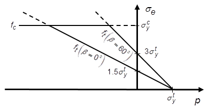
A composite yield surface is used to describe the different behavior in tension and compression. The tension behavior is pressure-dependent and the Rankine maximum stress criterion is used. The compression behavior is pressure-independent and the von Mises yield criterion is used. In principal stress space, the yield surface is a cylinder with a tension cutoff (cap). Figure 4.13: Cross-Section of Yield Surface shows a cross section of the yield surface on principal deviatoric-stress space and Figure 4.14: Yield Surface in the Meridional Plane shows the composite yield surface in the meridional plane.

The yield surface for tension and compression "regimes" are described by Equation 4–88 and Equation 4–89 (Chen and Han([332])).
The yield function for the tension cap is:
 | (4–88) |
and the yield function for the compression regime is:
 | (4–89) |
where:
 = hydrostatic pressure = hydrostatic pressure |
 = von Mises equivalent stress = von Mises equivalent stress |
 = deviatoric stress tensor = deviatoric stress tensor |
 = Lode angle = Lode angle |
 = second invariant of deviatoric stress
tensor = second invariant of deviatoric stress
tensor |
 = third invariant of deviatoric stress
tensor = third invariant of deviatoric stress
tensor |
 = tension yield stress = tension yield stress |
 = compression yield stress = compression yield stress |
Flow Rule
The plastic strain increments are defined as:
 | (4–90) |
where  is the so-called plastic flow potential, which
consists of the von Mises cylinder in compression and modified to
account for the plastic Poisson's ratio in tension, and takes the
form:
is the so-called plastic flow potential, which
consists of the von Mises cylinder in compression and modified to
account for the plastic Poisson's ratio in tension, and takes the
form:
 | (4–91) |
 | (4–92) |
where:

|
 = plastic Poisson's ratio (input
via TB,CAST) = plastic Poisson's ratio (input
via TB,CAST) |
 = flow potential in compression = flow potential in compression |
 = flow potential in tension = flow potential in tension
|
Experimental evidence suggests that  is always less than 0.5. For
  = 0.5, Equation 4–92 reduces to
the von Mises cylinder. The flow potentials in the meridional plane
are shown in this figure:
= 0.5, Equation 4–92 reduces to
the von Mises cylinder. The flow potentials in the meridional plane
are shown in this figure:
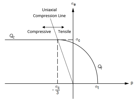
The region to the left of the uniaxial compression line is the compressive flow potential, while the region to the right is the tensile flow potential. As the flow potential is different from the yield function (nonassociated flow rule), the resulting material Jacobian is unsymmetric.
Hardening
The yield stress in uniaxial tension,  , depends on the equivalent uniaxial plastic strain
in tension,
, depends on the equivalent uniaxial plastic strain
in tension,  , and the temperature
  . Also the yield stress in uniaxial compression,
 , depends on the equivalent uniaxial plastic strain
in compression,
, depends on the equivalent uniaxial plastic strain
in compression,  , and the temperature
  .
.
To calculate the change in the equivalent plastic strain in tension, the plastic work expression in the uniaxial tension case is equated to general plastic work expression as:
 | (4–93) |
where:
 = plastic strain vector
increment = plastic strain vector
increment |
The change in the equivalent plastic strain in compression is defined as:
 | (4–94) |
where:

|