


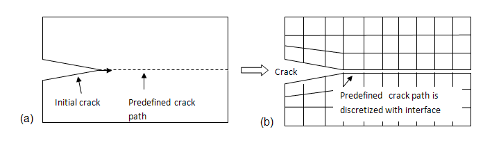
The virtual crack closure technique (VCCT) was initially developed to calculate the energy-release rate of a cracked body.[6] It has since been widely used in the interfacial crack-growth simulation of laminate composites, with the assumption that crack-growth is always along a predefined path, specifically the interfaces.[7][8][9][10]
VCCT-based crack-growth simulation is available with current-technology linear elements PLANE182 and SOLID185.
A VCCT-based crack-growth simulation involves the following assumptions:
Crack growth occurs along a predefined crack path.
The path is defined via interface elements.
The analysis is quasi-static and does not account for transient effects.
The material is linear elastic and can be isotropic, orthotropic or anisotropic.
The model undergoes small deformation (or small rotation) (NLGEOM,OFF).
The crack can be located in a material or along the interface of the two materials. The fracture criteria are based on energy-release rates calculated using VCCT. Several fracture criteria are available, including a user-defined option. Multiple cracks can be defined in an analysis.
A VCCT-based crack-growth simulation uses:
The CINT command to calculate the energy-release rate.
The CGROW command to define the crack-growth set, fracture criterion, crack-growth path, and solution-control parameters.
A VCCT-based crack-growth simulation is assumed to be quasi-static. Following is the general process for performing the simulation:
Crack-growth simulation is a nonlinear structural analysis. The analysis details presented here emphasize features specific to crack-growth.
Standard nonlinear solution procedures apply for creating a finite element model with proper solution-control settings, loadings and boundary conditions.
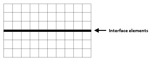
The predefined crack path is discretized with interface elements and grouped as an element component, as shown in the following figure:
The interface elements can be meshed via the CZMESH command or by a third-party tool that generates interface elements.
The element MPC constraint option (KEYOPT(2) = 1) bonds the potential crack faces together before cracks begin to grow. The MPC constraints are subsequently released when the fracture criterion is met, thus growing the cracks.
In a 2D problem, one interface element behind the crack tip may open if it meets the fracture criterion at a given substep. In a 3D problem, all interface elements behind the crack front may open if they meet the fracture criterion.
Differences in the size of the elements ahead of and behind the crack tip/front affect the accuracy of the energy-release rate calculation. While Mechanical APDL uses a correction algorithm, it may be inadequate to produce an accurate solution. Instead, use equal sized meshes for elements along the predefined crack path. For more information, see Calculating Fracture Parameters.
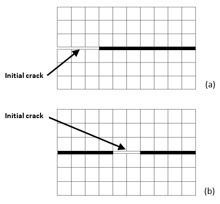
3.5.1.1.1. Generating Interface Elements via CZMESH
When using the CZMESH command to generate interface elements along the predefined crack path, add interface elements along the entire interface (including the initial crack and the predefined crack path), then delete interface elements on the initial crack:
For VCCT-based crack-growth simulation, it is necessary to perform the energy-release rate calculation first.
To calculate the energy-release rates, issue the CINT,TYPE,VCCT command. Issue subsequent CINT commands to specify other options such as the crack-tip node component and crack plane/edge normal.
The VCCT calculation uses the following assumptions:
The strain energy released when a crack advances by a small amount is the same as the energy required to close the crack by the same amount.
The crack-tip field/deformation at the crack-tip/front location is similar to when the crack extends by a small amount.
The assumptions do not apply when crack-growth approaches the boundary or when the two cracks approach each other; therefore, use the VCCT calculation with care and examine the analysis results.
For further information, see VCCT Energy-Release Rate Calculation.
The crack-growth calculation occurs in the solution phase after stress calculation. To perform the crack-growth calculation, you must define a crack-growth set, then specify the crack path, fracture criterion, and crack-growth solution controls. The solution command CGROW defines all necessary crack-growth calculation parameters.
Perform the crack-growth calculation as follows:
To define a crack-growth set,
issue the CGROW,NEW,n command,
where n is the crack-growth set number.
To define the crack path, issue the
CGROW,CPATH,cmname
command, where cmname is the component name for
the interface elements.
Specify the crack-calculation ID via
CGROW,CID,n, where
n is the crack-calculation
(CINT) ID for energy-release rate calculation with
VCCT. (The CINT command defines parameters associated
with fracture parameter calculations.)
For a simple fracture criterion such as the critical energy-release rate, you
can specify it by issuing
CGROW,FCOPTION,GC,VALUE,
where VALUE is the critical energy-release
rate.
For a more complex fracture criterion, you can specify the fracture
criteria via a material data table. Issue
CGROW,FCOPTION,MTAB,matid,
where matid is the material ID for the material
table. Several fracture criterion options are available (such as linear,
bilinear, B-K, modified B-K, Power Law, and user-defined).
For more information, see TB,CGCR and Fracture Criteria.
For each crack-growth set, you can specify only one fracture criterion, and one element component for crack-growth. You can define multicrack-growth sets with different cracks and fracture criteria. Multiple cracks can grow simultaneously and independently from each other. Cracks can merge to a single crack when they are on the same interface, as shown in the following figure:
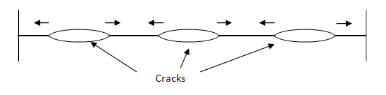
You can also define the same crack with different fracture criteria in a separate crack-growth set. The cracks can grow based on different criteria (according to which criterion is met), and are independent from each other. This technique is useful for comparing fracture mechanisms.
Issue the CGROW command to specify solution controls, as follows:
| To specify this solution control... | Issue this CGROW command: |
|---|---|
| Fracture criterion ratio (fc) |
CGROW,FCRAT, VALUE is the ratio. |
| Initial time step when crack-growth initiates |
CGROW,DTIME, VALUE is initial time
stepTo avoid over-predicting the load-carrying capacity, specify a small initial time step. |
| Minimum time step for subsequent crack-growth |
CGROW,DTMIN, VALUE is the minimum
time-step size. |
| Maximum time step for subsequent crack-growth |
CGROW,DTMAX, VALUE is the maximum
time-step size. |
| Maximum crack extension allowed at any crack-front nodes |
CGROW,STOP,CEMX, VALUE is the maximum crack
extension.Because crack-growth simulation can be time-consuming, use this command to stop the analysis when the specified crack extension of interest has been reached. |
When a crack extends rapidly (for example, in cases of unstable crack-growth), use smaller DTMAX and DTMIN values to allow time for load rebalancing. When a crack is not growing, the specified time-stepping controls are ignored and the solution adheres to standard time-stepping control.
The following input example defines a crack-growth set:
CGROW,NEW,1
CGROW,CPATH,cpath1
CGROW,FCOPTION,MTAB,5
CGROW,DTIME,1.0e-4
CGROW,DTMIN,1.0e-5
CGROW,DTMAX,2.0e-3
...
In a crack-growth simulation, a quantity of interest is the amount of crack extension. VCCT measures the crack extension based on the length of the interface elements that have opened, as expressed by the following equation and in the subsequent figure:

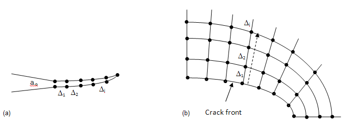
For 2D crack problems, the crack extension is the summation of length of interface elements that are currently open (a). For 3D problems, the crack extension is measured at each crack-front node and is the summation of the length of the interface element edges that follow the crack extension direction (b).
Crack extension  is available as CEXT as part of the crack solution variable
associated with the crack-calculation ID, and can be postprocessed similar to energy
release rates via POST1 and POST26 postprocessing commands (such
PRCINT, PLCINT, and
CISOL).
is available as CEXT as part of the crack solution variable
associated with the crack-calculation ID, and can be postprocessed similar to energy
release rates via POST1 and POST26 postprocessing commands (such
PRCINT, PLCINT, and
CISOL).
To model the crack-growth, it is necessary to define a fracture criterion for crack onset and the subsequent crack-growth. For linear elastic fracture mechanics (LEFM) applications, the fracture criterion is generally assumed to be a function of Mode I (GI), Mode II (GII), and Mode III ((GIII) critical energy-release rates, expressed as:

Other parameters may be necessary for some models.
Fracture occurs when the fracture criterion index is met, expressed as:

where fc is the fracture criterion ratio. The recommended ratio is 0.95 to 1.05. The default is 1.0.
The following fracture criteria are available:
The user-defined option requires a subroutine that you provide to define your own fracture criterion.
To initiate a fracture criterion table without the critical energy-release rate criterion, issue the TB,CGCR command.
The critical energy-release rate criterion uses total energy-release rate (GT) as fracture criterion. The total energy-release rate is summation of the Mode I (GI), Mode II (GII), and Mode III ((GIII) energy-release rates, expressed as:

where  is the critical energy-release rate.
For Mode I fracture, the fracture criterion reduces to:

The critical energy-release rate option is the simplest fracture criterion and is suitable for general 2D and 3D crack-growth simulation.
The linear option assumes that the fracture criterion is a linear function of the Mode I (GI), Mode II (GII), and Mode III ((GIII) energy-release rates, expressed as:

where  ,
,  , and
, and  are the Mode I, Mode II, and Mode III critical energy-release
rates, respectively. The three values are input via the
TBDATA command, as follows:
are the Mode I, Mode II, and Mode III critical energy-release
rates, respectively. The three values are input via the
TBDATA command, as follows:
| Constant | TBDATA Input | Comments |
|---|---|---|

|
C1
| Critical Mode I energy-release rate,  >= 0 >= 0 |

|
C2
| Critical Mode II energy-release rate,  >= 0 >= 0 |

|
C3
| Critical Mode III energy-release rate,  >= 0 >= 0 |
Example 3.9: Linear Criterion Input
g1c=10.0
g2c=20.0
g3c=25.0

TB,CGCR,1,,,LINEAR
TBDATA,1,g1c,g2c,g3c
The three constants cannot all be zero. If a constant is set to zero, the corresponding term is ignored.
When all three critical energy-release rates are equal, the linear fracture criterion reduces to the critical energy-release rate criterion.
The linear fracture criterion is suitable for 3D mixed-mode fracture simulation where distinct Mode I, Mode II, and Mode III critical energy-release rates exist.
The bilinear fracture option [8] assumes that the fracture criterion is a linear function of the Mode I (GI) and Mode II (GII) energy-release rates, expressed as:

where  and
and  are the Mode I and Mode II critical energy-release rates,
respectively, and ξ and ζ are the two material constants. All four
values can be defined as a function of temperature and are input via the
TBDATA command, as follows:
are the Mode I and Mode II critical energy-release rates,
respectively, and ξ and ζ are the two material constants. All four
values can be defined as a function of temperature and are input via the
TBDATA command, as follows:
| Constant | TBDATA Input | Comments |
|---|---|---|

|
C1
| Critical Mode I energy-release rate,  > 0 > 0 |

|
C2
| Critical Mode II energy-release rate,  > 0 > 0 |
| ξ |
C3
| ξ > 0 |
| ζ |
C4
| ζ > 0 |
Example 3.10: Bilinear Criterion Input
g1c=10.0
g2c=20.0
x=2
y=2

TB,CGCR,1,,,BILINEAR
TBDATA,1,g1c,g2c,x,y
The bilinear fracture criterion is suitable for 2D mixed-mode fracture simulation.
The B-K [7] option is expressed as:

where  and
and  are the Mode I and Mode II critical energy-release rates,
respectively, and η is the material constant. All three values can be
defined as a function of temperature and are input via the
TBDATA command, as follows:
are the Mode I and Mode II critical energy-release rates,
respectively, and η is the material constant. All three values can be
defined as a function of temperature and are input via the
TBDATA command, as follows:
| Constant | TBDATA Input | Comments |
|---|---|---|

|
C1
| Critical Mode I energy-release rate,  > 0 > 0 |

|
C2
| Critical Mode II energy-release rate,  > 0 > 0 |
| η |
C3
| η > 0 |
The B-K criterion is intended for composite interfacial fracture and is suitable for 3D mixed-mode fracture simulation.
The modified B-K (or Reeder) [9] option, is expressed as:

where  ,
,  , and
, and  are Mode I, Mode II, and Mode III critical energy-release
rates, respectively, and η is the material constant. All four values can be
defined as a function of temperature and are input via the
TBDATA command, as follows:
are Mode I, Mode II, and Mode III critical energy-release
rates, respectively, and η is the material constant. All four values can be
defined as a function of temperature and are input via the
TBDATA command, as follows:
| Constant | TBDATA Input | Comments |
|---|---|---|

|
C1
| Critical Mode I energy-release rate,  > 0 > 0 |

|
C2
| Critical Mode II energy-release rate,  > 0 > 0 |

|
C3
| Critical Mode III energy-release rate,  > 0 > 0 |
| η |
C4
| η > 0 |
When  =
=  , the modified B-K criterion reduces to the B-K criterion.
The modified B-K criterion is intended for composite interfacial fracture to account for distinct Mode II and Mode III critical energy-release rates, and is suitable for 3D mixed-mode fracture simulation.
Example 3.12: Modified B-K Criterion Input
g1c=10.0
g2c=20.0
g3c=25.0
h=2

TB,CGCR,1,,,MBK
TBDATA,1,g1c,g2c,g3c,h
The power law [10] option assumes that the fracture criterion is a power function of the Mode I (GI), Mode II (GII), and Mode III ((GIII) energy-release rates, expressed as:

where  ,
,  , and
, and  are Mode I, Mode II, and Mode III critical energy-release
rates, respectively, and n1, n2,
and n3 are power exponents and are also constants. All
six values can be defined as a function of temperature and are input via the
TBDATA command, as follows:
are Mode I, Mode II, and Mode III critical energy-release
rates, respectively, and n1, n2,
and n3 are power exponents and are also constants. All
six values can be defined as a function of temperature and are input via the
TBDATA command, as follows:
| Constant | TBDATA Input | Comments |
|---|---|---|

|
C1
| Critical Mode I energy-release rate,  > 0 > 0 |

|
C2
| Critical Mode II energy-release rate,  > 0 > 0 |

|
C3
| Critical Mode III energy-release rate,  > 0 > 0 |
| n1 |
C4
| n1 > 0 |
| n2 |
C5
| n2 > 0 |
| n3 |
C6
| n3 > 0 |
The three critical energy-release rates cannot all be zero. If a constant is set to zero, the corresponding term is ignored.
When power exponents n1, n2, and n3 are set to 1, the power law criterion is reduced to the linear fracture criterion.
The power law fracture criterion is suitable for 3D mixed-mode fracture simulation where distinct Mode I, Mode II, and Mode III critical energy-release rates exist.
Example 3.13: Power Law Criterion Input
g1c=10.0
g2c=20.0
g3c=25.0
n1=2
n2=2
n3=3

TB,CGCR,1,,,POWERLAW
TBDATA,1,g1c,g2c,g3c,n1,n2,n3
A custom fracture criterion that you define is expressed as:

where the fracture criterion is a function of the Mode I (GI), Mode II (GII), and Mode III (GIII) energy-release rates, and the material constant(s). All values are input via the TBDATA command.
A subroutine that you provide is necessary. For more information, see the Programmer's Reference.
Following is an example subroutine defining a linear fracture criterion:
*deck,user_cgfcrit      optimize
      SUBROUTINE user_cgfcrit (cgi,   cid,  kct,
     &                         nprop, prop, fcscl,
     &                         var1, var2, var3, var4)
c*****************************************************************
c
c *** primary function:
c              compute fracture criterion for crack-growth
c              user fracture criterion example
c
#include "impcom.inc"
#include "ansysdef.inc"
c
c     input arguments
c     ===============
c       cgi         (int,sc   , in)    CGROW set id
c       cid         (int,sc   , in)    CINT ID to be used
c       kct         (int,sc   , in)    Current crack-tip node
c       nprop       (int,sc   , in)    number of properties
c       prop        (dp ,ar(*), in)    property array
c
c     Output arguments
c     ===============
c       fcscl       (dp, sc   , ou)    fracture criterion
c                                      a return value of one or bigger
c                                      indicates fracture
c
c     Misc.  arguments
c     ===============
c       var1        (   ,     ,   )    not used
c       var2        (   ,     ,   )    not used
c       var3        (   ,     ,   )    not used
c       var4        (   ,     ,   )    not used
c
c*****************************************************************
c
c *** subroutines/function
c ***    get_cgfpar    : API to access fracture data
c ***    wrinqr        : ansys standard io function
c ***
      external         get_cgfpar
      external         wrinqr
      integer          wrinqr

c *** argument
c
      INTEGER          cgi, cid, kct, nprop
      double precision fcscl,
     &                 var1, var2, var3, var4
      double precision prop(nprop)
c
c *** local variable
c
      integer          debugflag, iott
      integer          nn
      double precision g1c, g2c, g3c, g1, g2, g3
      double precision gs(4),da(1)
c
c *** local parameters
      DOUBLE PRECISION ZERO, ONE
      parameter       (ZERO = 0.0d0,
     &                 ONE  = 1.0d0)
c
c*****************************************************************

c *** initialization
      fcscl = ZERO

c *** retrieve energy-release rates
c *** for crack cid and crack-tip node kct
c *** gs(1:3) will be returned as G1, G2, G3

c *** get energy-release rates
      nn  = 3
      gs(1:nn) = ZERO
      call get_cgfpar ('GS  ', cid, kct, 0, nn, gs(1))

c *** get crack extension
      nn = 1
      da(1)    = ZERO
      call get_cgfpar ('DA  ', cid, kct, 0, nn, da(1))

c *** energy-release rates
      g1 =abs(gs(1))
      g2 =abs(gs(2))
      g3 =abs(gs(3))

c *** input property from TBDATA,1,c1,c2,c3
      g1c   = prop(1)
      g2c   = prop(2)
      g3c   = prop(3)

c *** linear fracture criterion
      fcscl = ZERO
      if (g1c .gt. TINY) fcscl = fcscl + g1/g1c
      if (g2c .gt. TINY) fcscl = fcscl + g2/g2c
      if (g3c .gt. TINY) fcscl = fcscl + g3/g3c

c *** user debug output
      debugflag = 1
      if (debugflag .gt. 0) then
         iott = wrinqr (WR_OUTPUT)
         write(iott, 1000) cgi, cid, kct, da(1), fcscl, gs(1:3)
 1000 format (5x,'user fracture criterion:'/
     &  5x, 'crack-growth set ID           =',i5/
     &  5x, 'crack ID                      =',i5/
     &  5x, 'crack-tip node                =',i5/
     &  5x, 'crack extension               =',g11.5/
     &  5x, 'calculated fracture parameter =',g11.5/
     &  5x, 'energy-release rates Gs(1:3)  =',3g12.5)
      end if

      return
endThis example uses a double-cantilever beam with an edge crack at one end. Equal displacements with opposite directions are applied to the end of the beam about and below the crack in order to open up the crack, as shown in this figure:
Figure 3.19: Crack-Growth of a Double-Cantilever Beam
|
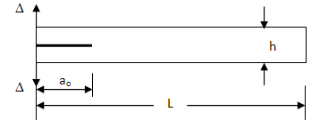 |


This figure shows the finite element mesh:

PLANE182 with the enhanced strain option (KEYOPT(1) = 2) is used to model the solid part of the model. INTER202 is used to model the crack path. A plane strain condition is assumed. In the vertical direction, the model uses 6 elements, and in the horizontal direction are 200 elements.
This figure shows the predicted load-deflection curve:
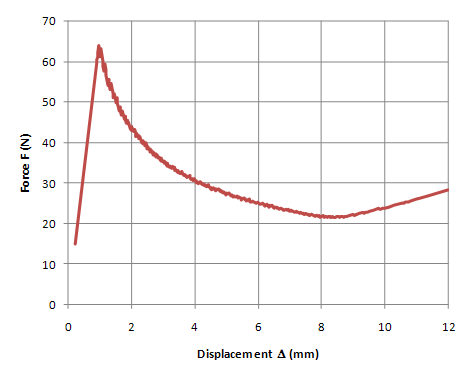
The force increases with the applied displacement and peaks quickly before the crack begins to grow. The reaction force then decreases rapidly at the initial phase of crack-growth, the slows down with the subsequent crack-growth. The results match very well with the reference results.[11]
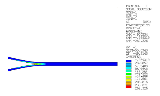
The contour plot of maximum principal stress is shown in the following figure:
Following is the input file used for the VCCT-based crack-growth simulation of the double-cantilever beam:
/prep7
dis1=0.9
dis2=12.0
n1=1000
n2=1000
n3=10
dl=100
dh=3
a0=30
nel=200
neh=6
toler=0.1e-5

et,1,182                   !* 2d 4-node structural solid element
keyopt,1,1,2               !* enhance strain formulation
keyopt,1,3,2               !* plane strain
et,2,182
keyopt,2,1,2
keyopt,2,3,2

et,3,202                   !* 2d 4-node cohesive zone element
!keyopt,3,2,2              !* element free option
keyopt,3,3,2               !* plane strain

mp,ex,1,1.353e5            !* e11 = 135.3 gpa
mp,ey,1,9.0e3              !* e22 =   9.0 gpa
mp,ez,1,9.0e3              !* e33 =   9.0 gpa
mp,gxy,1,5.2e3             !* g12 =   5.2 gpa
mp,prxy,1,0.24
mp,prxz,1,0.24
mp,pryz,1,0.46

g1c=0.28                   !* critical energy-release rate
g2c=0.80
g3c=0.80
tb,cgcr,1,,3,linear        !* linear fracture criterion
tbdata,1,g1c,g2c,g3c

! FE model
rectng,0,dl,dh/2           !* define areas
rectng,0,dl,0,-dh/2
lsel,s,line,,2,8,2         !* define line division
lesize,all,dh/neh
lsel,inve
lesize,all, , ,nel
allsel,all
type,1                     !* mesh area 2
mat,1
local,11,0,0,0,0
esys,11
amesh,2
csys,0
type,2                     !* mesh area 1
esys,11
amesh,1
csys,0
nsel,s,loc,x,a0-toler,dl
nummrg,nodes
esln
type,3
mat,5
czmesh,,,1,y,0,            !* generate interface elements
allsel,all
nsel,s,loc,x,dl            !* apply constraints
d,all,all
nsel,all

!
esel,s,ename,,202          !* select interface element to
cm,cpath,elem              !* define crack-growth path

nsle
nlist
nsel,s,loc,x,a0
nsel,r,loc,y,0
nlist
esln
elist
cm,crack1,node            !* define crack-tip node component
nlist
alls
finish

/solu
resc,,none
esel,s,type,,2
nsle,s
nsel,r,loc,x
nsel,r,loc,y,dh/2        !* apply displacement loading on top
d,all,uy,dis1
nsel,all
esel,all
esel,s,type,,1
nsle,s
nsel,r,loc,x
nsel,r,loc,y,-dh/2         !* apply displacement loading on bottom
d,all,uy,-dis1
nsel,all
esel,all
autots,on
time,1

cint,new,1            !* crack id
cint,type,vcct        !* vcct calculation
cint,ctnc,crack1      !* crack-tip node component
cint,norm,0,2

! crack-growth simulation set
cgrow,new,1          !* crack-growth set
cgrow,cid,1          !* cint id for vcct calculation
cgrow,cpath,cpath    !* crack path
cgrow,fcop,mtab,1    !* fracture criterion
cgrow,dtime,2e-3
cgrow,dtmin,2e-3
cgrow,dtmax,2e-3
cgrow,fcra,0.98
nsub,4,4,4
allsel,all
outres,all,all
solve
time,2
esel,s,type,,2
nsle,s
nsel,r,loc,x
nsel,r,loc,y,dh/2          !* apply displacement loading on top
d,all,uy,dis2
nsel,all
esel,all
esel,s,type,,1
nsle,s
nsel,r,loc,x
nsel,r,loc,y,-dh/2         !* apply displacement loading on bottom
d,all,uy,-dis2
nsel,all
esel,all

nsubst,n1,n2,n3
outres,all,all
solve                      !* perform solution
finish

/post1
set,last
prci,1
!
set,1,4
plnsol,s,1
!
finish

/post26
nsel,s,loc,y,dh/2
nsel,r,loc,x,0
*get,ntop,node,0,num,max
nsel,all
nsol,2,ntop,u,y,uy
rforce,3,ntop,f,y,fy
prod,4,3, , ,rf, , ,20
/title,, dcb: reaction at top node verses prescribed displacement
/axlab,x,disp u (mm)
/axlab,y,reaction force r (n)
/yrange,0,60
xvar,2
prvar,uy,rf
prvar,2,3,4
/com,
finish
VCCT-based crack-growth simulation is available only with current-technology linear elements PLANE182 and SOLID185.
These assumptions apply to VCCT-based crack-growth simulation:
The material is linearly elastic, and can be isotropic, orthotropic, or anisotropic.
The analysis is assumed to be quasi-static. Although a transient analysis is possible, the fracture calculations do not account for the transient effects.
The VCCT-based mixed-mode energy-release rates calculation assumes that the crack-tip field / deformation at the crack-tip/front location is similar to when the crack extends by a small amount. This assumption does not apply when crack-growth approaches the boundary or when two cracks are close; therefore, use the VCCT calculation with care and examine the analysis results.
When fracture parameters in addition to CINT,VCCT are calculated on the same geometric crack front (for example, when both JINT and VCCT are requested on the same crack front), these limitations apply:
Distributed-memory parallel processing is no longer supported.
The additional parameter values become inaccurate as soon as the crack starts to grow.