All actuators can be conditional. See Condition to create this condition.

Measure that stores the evaluation of the actuator variable. Can be useful when the applied value depends on a measure other than time.

Measure that stores the energy generated by the actuator.

variable is a list of input measures in table form.

measure is typically the time measure object, but other measures can be used as well. When using an expression to define a load variation, the measure must have only one component (it cannot be a vector measure). The variation can be defined by a constant, an expression, or a table.

value is a Python float constant. See Relation object for defining a constant.

table is a CS_Table .

string is similar to the expression used in the user interface to define a joint condition by a function. Note that the literal variable is always called time, even if you are using another measure as input.

is_degree is a boolean argument. If the expression uses trigonometric function, it specifies that the input variable should be expressed in degrees.

Sets or gets function of the transformation matrix

Name of the body.

Origin Coordinate System of the body. This Coordinate System is the moving coordinate system of one of the joints connected to the body. The choice of this joint, called parent joint, is the result of an optimization that minimizes the number of degrees of freedom of the system.

Inertia body coordinate system of the body.

Type of body, values in E_UnknownType, E_Ground, E_Rigid, E_CMS, E_General, E_Fictitious, E_RigidLeaf, E_RigidSubModel, E_PointMass, E_Beam

Overwrites the mass and inertia values of a body.

Overwrites the position of the center of mass and the orientation of the inertia coordinate system.

Overwrites the constant mass and principal inertia properties by variable properties. During the solution process, the mass and inertia variation rate needs to be evaluated. Therefore, only Point Table, Polynomial and Function can be used to define the variation. Python user tables cannot be used to define kinetic properties variations. You can make some of the properties (mass, Ixx, Iyy and Izz) constants by using constant variables.

This function only applies to rigid bodies.

CS_FlexibleBody

Rotates the transient values of a measure to a coordinate system. MeasureValues is a python two-dimensional array, such as that coming out of FillValuesThroughTime or FillDerivativesThroughTime. This function works for 3D vectors such as relative translation between two coordinate systems or 6-D vectors such as forces/moments.

Rotates the transient values of a measure from a coordinate system to the global coordinate system.

Type of coordinate system, values in E_Unknown, E_Ground, E_Part, E_Joint, E_Inertia, E_BodyTransform, E_Contact, E_SplitJoint.

The ID of the condensed part in the Mechanical tree.

The vector of the IDs of the Mechanical parts that are used in the condensed part.

Retrieves a measure that contains the total contact force between the two linked bodies.

Enable output of contact points information specified by flag.

Disable output of contact points information specified by flag.

Time in second (=30.0 by default)

Enable verbose mode in contact.out file (=0, disabled by default)

Number of parallel threads used for contact detection (=2 by default)

Creation of a joint driver, on joint joint, degree of freedom components, and with motion type driverMotionType. Note that the same driver can prescribe more than one joint motion at the same time. This is useful if you want to add the same condition to all components of a prescribed motion for example. Components must be ordered, are zero based, and refer to the actual free degrees of freedom of the joint.

Corresponding system.

Example:

Env=CS_Environment.FindFirstNonNull()
Sys = Env.System

Ground body.

Example:

Env = CS_Environment.FindFirstNonNull()
Ground = Env.Ground

The vector of existing loads. This includes Springs that are considered by the solver as loads, as well as force and torque joint conditions.

Example:

Xdof = 0
Friction=CS_JointDOFLoad(PlanarJoint,Xdof)
Env.Loads.Add(Friction)

The vector of Body Loads.

Example:

MyBodyLoad = CS_BodyLoad()
…
Env.BodyLoads.Add(MyBodyLoad)

The vector of external constraint equations.

Example:

rel3=CS_Relation()
rel3.MotionType=CS_Relation.E_MotionType.E_Velocity

var30=CS_ConstantVariable()
var30.SetConstantValues(System.Array[float]([0.]))

var31=CS_ConstantVariable()
var31.SetConstantValues(System.Array[float]([23.]))

var32=CS_ConstantVariable()
var32.SetConstantValues(System.Array[float]([37.]))

var33=CS_ConstantVariable()
var33.SetConstantValues(System.Array[float]([-60.+37.]))

rel3.SetVariable(var30)
rel3.AddTerm(jp,0,var31)
rel3.AddTerm(js3,0,var32)
rel3.AddTerm(jps,0,var33)

Env.Relations.Add(rel3)

The vector of Displacements, Velocity and Acceleration joint conditions.

The vector of Displacements, Velocity, and Acceleration joint conditions to be used only at time=0.

Gets the Potential Energy Measure.

Gets the Kinetic Energy Measure.

Gets the Total Energy Measure.

Gets the Actuator Energy Measure.

Specifies the starting time in a restart analysis

Returns the first environment in the global list. The table usually contains only one environment, thus it is a common way to access the current environment.

Example:

Env=CS_Environment.FindFirstNonNull()

Overwrites the end time of the simulation.

Solves the current analysis.

Uses a variable to define the amount of alpha Rayleigh damping (proportional to the mass matrix) to be considered for the flexible body. The variable can be either dependent or constant.

Example:

aFlexibleBody.AlphaDamping=100

Or equivalently:

var=CS_Variable()
var.SetConstantValues(System.Array[float]([100.]))
aFlexibleBody.AlphaDamping=var

Uses a variable to define the amount of beta Rayleigh damping (proportional to the mass matrix) to be considered for the flexible body. The variable can be either dependent or constant.

Example:

Env=CS_Environment.GetDefault()
Sys=Env.System
 
array=System.Array.CreateInstance(float,4,2)
array[0,0]=0.0
array[0,1]=5.e-6
array[1,0]=0.05
array[1,1]=5.e-6
array[2,0]=0.051
array[2,1]=1.e-4
array[3,0]=0.1
array[3,1]=1.e-4
 
table=CS_PointsTable(array)
 
(err,found,time)=Sys.FindOrCreateInternalMeasure(CS_Measure.E_MeasureType.E_Time)
 
var=CS_Variable()
var.AddInputMeasure(time)
var.SetTable(table)
 
aFlexibleBody.BetaDamping = var

Define a factor to be used to multiply the default damping matrix. For instance, with a CMSBody, this matrix can be created during the generation pass. When the damping matrix is generated for a Condensed Part (CMSBody), it will be automatically taken into account in the RBD use pass with a factor equal to 1.0.

Define the amount of damping used for the degree of freedom specified by iDof (index starts at 0). The variable can be either dependent or constant.

Retrieve the damping variable defined for the degree of freedom iDof (index starts at 0).

Define a scale factor applied to the flexible body internal load specified by iLV (index starts at 0). By default, the first load vector uses a constant scale factor equal to 1.0.

Retrieve the variable associated to the factor specified by iLV (index starts at 0).

Creates a GIL table with sizeIn inputs and sizeOut outputs

Creates a GIL table from a text file; filename is the name of the file containing the points (typically a .CSV file). This file must be in ASCII format, with one data point per row. Each row must contain sizeIn + sizeOut columns. The columns must be separated by a character specified by the argument separator. The default value of separator is ,. scale is an optional argument that scales all the output values. The default value, used if the optional argument is not specified, is 1.0. noHeader is a boolean, optional argument that should be true if there is no first row with labels.

Example file:

Velocity, Deflection, Force
0.,0.,10.0
100.,0.,200.0
...

Adds an interpolation point to the General Interpolation Table. values is a one dimensional array of size sizeIn+sizeOut. The first sizeIn values in array values corresponds to the values of the input variables. The following sizeOut values in array values correspond to the output values.

VarForceY = CS_Variable();
#
# Variable 0: spin
VarForceY.AddInputMeasure(SpinMeasure )
#
# Variable 1: Y displacement
VarForceY.AddInputMeasure( TransY )
# 
# Create table with 2 input and 1 output
EvalY = CS_GILTable(2,1)

Omega = -1.0
dY = -1e-4
stiff = -9.0

values=System.Array.CreateInstance(float,3)

values[0] = Omega
values[1] = dY
values[2] = stiff
EvalY.AddInterpolationPoint( values )

Omega = 11.0
dY = -1e-4
stiff = -21.0
values[0] = Omega
values[1] = dY
values[2] = stiff
EvalY.AddInterpolationPoint( values )
…

Adds a set of points to the General Interpolation Table. values is a two dimensional array of size (numberOfPoints, sizeIn+sizeOut). On each row of the array, first sizeIn values in array values corresponds to the values of the input variables. The following sizeOut values in array values correspond to the output values. Each row contains a single interpolation point in the cloud of points.

ForceVariable = CS_Variable()
ForceVariable.AddInputMeasure( TransX )
Evaluator = CS_GILTable( 1,1 )
values = System.Array.CreateInstance( float, 6, 2 )
dX = 0.0
F = 0.0
values[0,0] = dX
values[0,1] = F

dX = 10.0
F = 1.0
values[1,0] = dX
values[1,1] = F

dX = 30.0
F = 2.0
values[2,0] = dX
values[2,1] = F

dX = 60.0
F = 3.0
values[3,0] = dX
values[3,1] = F

dX = 90.0
F = 4.0
values[4,0] = dX
values[4,1] = F

dX = 130.0
F = 5.0
values[5,0] = dX
values[5,1] = F
Evaluator.AddInterpolationPointArray( values ) 

If bVerbose is set to true, the GILTable will print the output value every time it is evaluated. This can be used for debugging purposes, but it will affect the performance if used on a table in a long simulation.

Name of the joint

Joint reference coordinate system

Example:

J1 = CS_Joint.Find(_jid)
CSR = J1.ReferenceCoordinateSystem

Joint moving coordinate system

Example:

J1 = CS_Joint.Find(_jid)
CSM = J1. MovingCoordinateSystem

Joint type

The internal representation of the joint can use flipped reference and mobile coordinate systems. In that case, all the joint results (for example, forces, moments, rotation, velocities and acceleration) must be multiplied by -1 to go from their internal representation to the user representation. As transient values of joint measures are giving the internal representation, use this IsRevert information to know if results should be negated.

When extracting joint degrees of freedom on joints that return true, accelerations should be done using the time derivatives of the joint velocity measure. On joints that return false, joint DOF derivatives should be extracted using the joint acceleration measure. It is important to check this flag first. Use of the wrong method to query joint acceleration can result in failure or incorrect results.

Example:

if Universal.AccelerationFromVelocitiesDerivatives:
	UniversalAccelerationValues=UniversalVelocityM.FillDerivativesThroughTime()
else:
	UniversalAcceleration = Universal.GetAcceleration()
	UniversalAccelerationValues=UniversalAcceleration.FillValuesThroughTime()

Returns the list of the stops defined on the joint.

Returns the joint velocity measure. The size of this measure is the number of degrees of freedom of the joint. The derivatives of this measure give access to the joint accelerations.

Returns the joint rotation measure. The type of measure depends on the joint number of rotational degrees of freedom (E_1DRotationMeasure, E_3DRotationMeasure, E_UniversalAngles). These rotations components are relative to the reference coordinate system of the joint.

Returns the joint translation measure. The length of this measure is the number of translational degrees of freedom of the joint. The translation components are expressed in the reference coordinate system of the joint.

Returns the joint force measure. The length of this measure is always 6 (3 forces components, 3 torque component). This force measure is the total force/moment, including constraint forces/moment, external forces/moment applied to the joint, and joint internal forces/moment, such as elastic moment in a revolute joint that has a stiffness on the Z rotation axis. The force measure components are expressed in the global coordinate system. Note that the sign convention is different from the sign convention used in the Joint Probes in Mechanical.

Returns the joint acceleration measures on the joints that are constraint equations based. See the AccelerationFromVelocitiesDerivatives member to see when this function should be used.

Example:

J1 = CS_Joint.Find(_jid)
jointRotation = J1.GetRotation()
jointVelocity = J1.GetVelocity()
jointAcceleration = J1.GetAcceleration()
jointForce = J1.GetForce()

Replaces the constant value already given to the friction coefficient with the expression given by var.

Example:

Joint = CS_Joint.Find(_jid)
Var = CS_Variable()
u0 = 0.1
u1 = 0.2
alpha = 0.5
Var.SetFunc('u0+u1exp(-alpha*time)',0)
Var.AddInputMeasure(Joint.GetVelocity())
Joint.SetFrictionVariable(Var)

The command has no effect if no value for the friction coefficient has been provided in the UI. For more information, see Joint Friction

Sets the friction tolerance.

Example:

Joint = CS_Joint.Find(_jid)
Joint = Joint.SetFrictionTolerance(1e-4)

A joint object

An integer that defines the joint degree of freedom to be included in the term. The ordering of the degrees of freedom sets the translation degrees of freedom first. The degrees of freedom numbering is zero based. For example, in a slot joint, the translational degree of freedom is 0, while the third rotational degree of freedom is 3.

Number of components of the measure

Example:

nbValues = Measure.Length

Measure type

A measure can use direct calculation or be time integrated. On a measure that uses direct calculation, it is possible to retrieve the measure value through time. On a measure that is time-integrated, both values and time derivatives can be retrieved.

Measure Name

Returns a two dimensional array. This function is to be called after the solution has been performed. The first dimension of the returned array is the number of time values in the transient. The second dimension is the size of the measure plus one. The first column contains the time values, while the subsequent columns contain the corresponding measure values.

Example:

jointRotation = J1.GetRotation()
jointVelocity = J1.GetVelocity()
jointAcceleration = J1.GetAcceleration()
jointForce = J1.GetForce()

jointRotationValues =jointRotation.FillValuesThroughTime()
jointVelocityValues =jointVelocity.FillValuesThroughTime()
jointAccelerationValues =jointAcceleration.FillValuesThroughTime()
jointForceValues =jointForce.FillValuesThroughTime()

nbValues = jointRotationValues.GetLength(0)

print jointRotation.Id

print '  Time     Rotation Velocity Acceleration'
for i in range(0,nbValues):
    print jointRotationValues[i,0],jointRotationValues[i,1],jointVelocityValues[i,1],jointAccelerationValues[i,1]

fich.close()

Returns a two dimensional array. This function is to be called after the solution has been performed. The first dimension of the returned array is the number of time values in the transient. The second dimension is the size of the measure plus one: the first column contains the time values, while the subsequent columns contain the corresponding measure derivatives. These derivatives are available on measures that are time integrated. To know if a measure is time integrated, use the CalculationMethod member.

Both translational and rotational joint velocities are expressed in the joint reference coordinate system. The number of components is the number of translational degrees of freedom plus the number of rotational degrees of freedom. For example, the size of the joint velocity measure for a revolute joint is 1. It contains the relative joint rotation velocity along the z axis of the joint reference coordinate system. The size of the measure for a slot joint is 4: one component for the relative translational velocity, and the 3 components of the relative rotational velocity. The joint velocity measure can be obtained from the joint using the GetVelocity function. Rotational velocities are expressed in radians/second.

Both translational and rotational joint accelerations are expressed in the joint reference coordinate system. The number of components is the number of translational degrees of freedom plus the number of rotational degrees of freedom. The joint acceleration measure can be obtained from the joint using the GetAcceleration function.

This measure contains only the joint relative translations, expressed in the joint reference coordinate system. The joint translation measure can be obtained from the joint using the GetTranslationfunction.

This measure contains the total forces and moment that develop in the joint. This includes constraint forces, elastic forces, and external forces. The joint velocity measure can be obtained from the joint using the GetForcefunction.

This measure allows for tracking of the position of a Body Coordinate System over time.

Example:

CoMBCS = OneBody.InertiaBodyCoordinateSystem
Pos = CS_PositionMeasure(CoMBCS)
Env=CS_Environment.FindFirstNonNull()
Sys = Env.System
Sys.AddMeasure(Pos)

This measure allows the extraction of one component of an existing measure. This component can be expressed in a non default coordinate system. A component of -2 will compute the norm 2 of the vector of values of the measure.

Example:

Planar = CS_Joint.Find(_jid)
Vel = Planar.GetVelocity()
Xglobaldirection = 0
VelX = CS_ComponentMeasure(Vel,Xglobaldirection)
Sys.AddMeasure(VelX)

This measure allows a linear transformation from another measure with a scaling factor and an offset. This can be useful to transform an internal rotation measure that is expressed in radians to a measure in degrees used as an input to a load calculation, for example.

Example:

Revolute = CS_Joint.Find(_jid)
Rot = Revolute.GetRotation()
RotInDegrees = CS_AXPYMeasure( Rot, 180.0/math.pi, 0. )
Sys.AddMeasure(RotInDegrees)

This measure allows you to compute the floating point remainder of value/modulus.

Example:

Revolute = CS_Joint.Find(_jid)
Rot = Revolute.GetRotation()
Rot02pi = CS_ModulusMeasure( Rot, 2.0*math.pi )
Sys.AddMeasure(Rot02pi)

This measure contains four 3D vectors:

This measure computes the Angular Momentum of a list of bodies. Its value is a 3D vector.

Example:

FlyWheel= CS_Body.Find(_bid)
FlyWheelAngularMomentumMeasure = CS_AngularMomentumMeasure()
FlyWheelAngularMomentumMeasure.AddBody(FlyWheel)
Sys.AddMeasure(FlyWheelAngularMomentumMeasure)

Set the database file name.

Set the database directory.

Read the content of the database.

Write the current database to a file.

Delete the database.

Close the database file.

Open the database file and reads the database content table.

Clear the content of the database and free memory used by the database.

tab is a two dimensional array where the first column contains the input values and the second column contains the corresponding output values.

Example:

tab = System.Array.CreateInstance(float,6,2)
tab[0,0]=-100.
tab[1,0]=-8.
tab[2,0]=-7.9
tab[3,0]= 7.9
tab[4,0]= 8.
tab[5,0]= 100.

tab[0,1]=1.0
tab[1,1]=1.0
tab[2,1]=0.1
tab[3,1]=0.1
tab[4,1]=1.0
tab[5,1]=1.0
Table = CS_PointsTable(tab);

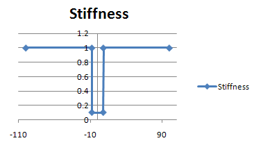
Here, the output (shown as Stiffness in the chart above) varies in a linear, piece-wise manner. For values of input less than -8.0 or greater than 8.0, the output is equal to 1.0. For values between -7.9 and +7.9, the output is 0.1. The transition is linear between -8.0 and -7.9, and as well between +7.9 and +8.0.

Creates an empty polynomial table.

Specialized for 1x1 table. Initializes the table to be a 1 input, 1 output table, and sets the constant term (constant is a float value).

(generic version) Initializes the table with sizeIn inputs and sizeOut outputs and sets the constant terms. sizeIn and sizeOut are two integer values, and constantValues is an array of sizeOut float values.

Specialized for 1x1 table. Adds one monomial term to the table. The coefficient is a float value and order is an integer value giving the power of the input.

(generic version) Adds one monomial term to the table. The coefficients are given by a sizeOut float array and the power for each input by an array of sizeIn integers.

Type of relation, with type selected in the previous enumeration.

Adds a term to the equation.

Sets the right hand side of the relation. "variable" is a variable object.

Multiplicative factor used to determine zero velocity tolerance (=100.0 by default);

Contact radius factor used in contact failsafe mode (=2.0 by default);

Number of external loops for geometric correction (=2 by default));

Enable friction for shock solve (=0, disabled by default);

Number of diagnostics messages given in Mechanical UI (=10 by default);

Prevent inactive contact pair from being violated (=1, enabled by default);

Disable polygon event for contact (=0, active by default);

Print the dynamics system (=0 by default);

Purge GST file every n steps (=0, never by default);

Force output of error estimation (=0, disabled by default);

Export generalized coordinates for CMS bodies in a CSV file (=0, disabled by default)

When point on curve joints are used, different solutions (depending on the topology) may be found when crossing curve connections. Furthermore, these solutions do not guarantee the conservation of the kinetic energy at the transition. To remedy this issue, this option makes the transitions using a method that minimizes the kinetic energy in a way similar to the assembly process using the inertia matrix. This solution works well for explicit time integration schemes, but it is not guaranteed for implicit ones. (=0, disabled by default)

Calling this function on a translational spring will make the spring develop elastic forces only if its length is less than the spring free length. The free length has to be defined in the regular spring properties.

Calling this function on a translational spring will make the spring develop elastic forces only if its length is greater than the free length of spring. The free length has to be defined in the regular spring properties.

Enables you to overwrite the stiffness and free length of a translational spring. This can be useful to parameterize these properties. For example, system is the system object, stiffness and free length are the double precision values of stiffness and free length.

Enables you to replace the constant stiffness of a spring with a table of ID table_id that gives the force as a function of the elongation of the spring. The table gives the relation between the force and the relative position of the two ends.

The user interface has stiffness and damping properties of the spring. Internally, the Spring is made of two objects; a spring and a damper. This function enables you to access the internal damper using the Spring object in the GUI.

Gets the list of bodies.

Gets the list of joints.

Adds a body to the system.

Adds a joint to the system.

Prints the topology of the systems (parent/child relation).

Adds a measure to the system, to be calculated during the simulation. This function must be called prior to solving so that the measure values through time can be retrieved.

Extracts an existing global measure on the system. Supported measure types are: E_Energy, E_PotentialEnergy, E_ElasticEnergy, E_KineticEnergy, and E_Time.

Allows evaluating a table in Python. In and Out are arrays of float, with sizes corresponding to the table input and output sizes. This function can be called from a user table for example.

Explicit destruction of the table. This explicit destructor should be used only when the table hasn’t been assigned to an actuator. When the table is assigned to an actuator, the actuator is calling this destructor. Omitting to call this destructor can cause the evaluation of the results to fail.

value is an array, whose size is equal to the size of the table. To create a constant scalar variable, the value can be defined as shown in the following example:

System, Array, and float are part of the Python language. The result of this is an array of size one, containing the value 1.0.

measure is a measure object. The same variable can have more than one measure. The input variable of the variable is formed by the values of the input measure in the order that they have been added to the list of input measures.

table is a CS_PointsTable.

string is similar to the expression used in the user interface to define a joint condition by a function. Note that the literal variable is always called "time", even if you are using another measure as input. "is_degree" is a boolean argument. If the expression uses a trigonometric function, it specifies that the input variable should be expressed in degrees.