3.2.2. Interaction Type Properties for Body Interaction Object

This section includes descriptions of the interaction types for the Body Interaction object:

Note: Only these four types of contact are permitted for Explicit Dynamic analyses.

3.2.2.1. Frictionless Type

Setting Type to Frictionless activates frictionless sliding contact between any exterior node and any exterior face of the scoped bodies. Individual contact events are detected and tracked during the analysis. The contact is symmetric between bodies (that is, each node will belong to a target face impacted by adjacent contact nodes; each node will also act as a contact impacting a target face).

Supported Connections

Explicit Dynamics

Connection Geometry	Volume	Shell	Line	Particle
Volume	Yes	Yes	Yes	Yes
Shell	Yes	Yes	Yes	Yes
Line	Yes	Yes	Yes^[a]	No
Particle	Yes	Yes	No	No

^[a]Only for Contact Detection = Proximity Based, and Edge on Edge Contact = Yes (This option switches on contact between ALL lines / bodies / edges; that is, there is no dependence on the scoping selection of body interactions)

LS-DYNA

Connection Geometry	Volume	Shell	Line	Particle
Volume	Yes	Yes	No	Yes
Shell	Yes	Yes	No	Yes
Line	No	No	No	No
Particle	Yes	Yes	No	No

3.2.2.2. Frictional Type

Setting Type to Frictional activates frictional sliding contact between any exterior node and any exterior face of the scoped bodies. Individual contact events are detected and tracked during the simulation. The contact is symmetric between bodies (that is, each node will belong to a target face impacted by adjacent contact nodes; each node will also act as a contact impacting a target face).

Friction Coefficient: A non-zero value will activate Coulomb type friction between bodies (F = μR).

The relative velocity (ν) of sliding interfaces can influence frictional forces. A dynamic frictional formulation for the coefficient of friction can be used.

(3–3)

where

= friction coefficient

= dynamic coefficient of friction

β = exponential decay coefficient

ν = relative sliding velocity at point of contact

Non-zero values of the Dynamic Coefficient and Decay Constant should be used to apply dynamic friction.

Supported Connections

Explicit Dynamics

Connection Geometry	Volume	Shell	Line	Particle
Volume	Yes	Yes	Yes	Yes
Shell	Yes	Yes	Yes	Yes
Line	Yes	Yes	Yes^[a]	No
Particle	Yes	Yes	No	No

LS-DYNA

Connection Geometry	Volume	Shell	Line	Particle
Volume	Yes	Yes	No	Yes
Shell	Yes	Yes	No	Yes
Line	No	No	No	No
Particle	Yes	Yes	No	No

3.2.2.3. Bonded Type

Setting Type to Bonded activates bonded contact between exterior nodes and exterior faces of the scoped bodies or regions. The node-face pairs that are considered to be bonded during the simulation are detected at initialization. During the analysis the node in each node-face pair is kept at the same relative position to the face to which it is bonded. This is done by means of penalty forces which can be dependent on either the mass of the nodes/faces or the stiffness of the material.

The Bonded Contact Region options pertinent to an Explicit Dynamics analysis are discussed in the remainder of this section.

Maximum Offset

The Maximum Offset value specifies the tolerance used at initialization to determine whether a node is bonded to a face. This is done using an automatic search algorithm which searches for the minimum distance from a node in a bonded region to all of the faces in the bonded region. If this minimum distance falls within the Maximum Offset value, the bond pair will be established. In order to compute the proper distance to a face the algorithm will determine if the perpendicular projection to the face falls within the face. If that is not the case, the perpendicular projection to the face edges is considered. If that is not the case, the distance to one of the face nodes is considered. This algorithm guarantees that a minimum distance is always found and can be properly compared against the value input for Maximum Offset.

Note: It is important to select an appropriate value for the Maximum Offset. The automatic search will bond everything together which is found within this value using the method described above. Therefore, it is important to ensure that the Maximum Offset it is not so large as to generate undesired bonded node-face pairs. Also, particular attention to the Maximum Offset value may be needed when setting up bonds including bodies with Reference Frame of type Particle. In this case, ensure that the Maximum Offset is large enough to capture the desired Particle nodes which may be half a particle diameter from the geometry exterior surface, but not too large such that undesired particles are bonded.

You can use the custom variable BOND_STATUS to check the bonded node-face pairs in an Explicit Dynamics analysis (not available in LS-DYNA analyses). This variable records the number of nodes bonded to the faces on an element during the analysis. This can be used to verify that the Maximum Offset is set appropriately in order to generate the desired bonded node-face pairs.

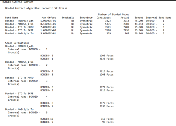
In addition to the BOND_STATUS variable, additional verification of the initialized bonds can be done by inspection of the prt file. A summary is given which lists the number of candidate nodes for bonding and the actual number of nodes that were bonded. If the percentage of nodes to be bonded is 0% it means none of the nodes are actually bonded. You should consider increasing the Maximum Offset in this case.

Breakable

If the Breakable option is set to No, then the bonds generated at initialization will be active for the entire analysis.

If the Breakable option is set to Stress Criteria, then the bond may break (or be released) during the analysis. The criteria for breaking a bond is defined as:

(3–4)

where

= the value entered for Normal Stress Limit

n = the value entered for Normal Stress Exponent

= the value entered for Shear Stress Limit

m = the value entered for Shear Stress Exponent

In Explicit Dynamics analyses, the BOND_STATUS variable can be used to identify bonds that have broken during the simulation.

Behavior

The Behavior option can be used as described in Behavior with some of the exceptions as discussed below..

In an Explicit Dynamics analysis Auto Asymmetric behavior is dependent on the type of scoping:

Bonded connections with only faces scoped will behave symmetrically.
All other bonded connections (if the Contact or Target is scoped to a vertex or edge) will behave asymmetrically.

Note that the generation of bonded node-face pairs at initialization is also dependent on the Behavior option:

Internal out-of-plane tolerance

For symmetric bond behavior the perpendicular projection of a node to a face has to fall within the face bounds otherwise the bond pair is disregarded a candidate.
For asymmetric bond behavior the perpendicular projection of a node to a face does not have to fall within the face bounds in order to be considered as a candidate.
For both types of behavior the Maximum offset is always taken into account.
If needed, a symmetric bond definition can also be changed to search out-of-plane by taking the following steps:
- Set the definition to Asymmetric in order to search out-of-plane
- Duplicate the definition of the bond object (right-click operation)
- Subsequently "flip" Contact and Target (right-click operation)
Effectively, you have created a symmetric definition (Contact->Target, Target->Contact) and bonds will be searched out of plane.

Bond definitions referring to a single part

Symmetric bonds are disregarded for definitions that scope to a single part.
Asymmetric bonds are considered for definitions that scope to a single part.

Trim Contact

The Trim Contact option is ignored by the Explicit solver.

Calculation of Penalty Forces

During the analysis the nodes are kept at the same relative position on the face to which they are bonded. This is done by means of penalty forces which are either dependent on the mass of the nodes/faces or the stiffness of the material. The stiffness is weighted based on materials on either side of the bond. In models with mass scaling the penalty method is chosen based on the mass scaling setting:

Mass scaling off: Penalty method based on harmonic mass in the bonded pair.
Mass scaling on: Penalty method based on harmonic stiffness in the bonded pair.

Origin of Model	Mass Scaling Off	Mass Scaling On
Any Workbench project opened in R18.0 or later	Harmonic Mass	Harmonic Stiffness

Note: The stiffness weighted penalty method is typically superior to a mass weighted penalty and increases the robustness of (offset) bonds. By switching on mass scaling and still using a small target timestep (eg 1e-20) no mass will be added, but the penalty method will be switched to harmonic stiffness.

When large material stiffness occurs between two materials that are bonded, it is recommended that you use an asymmetric definition where the contact scope (nodes to be bonded) refers to the soft material and the target scope (faces to bond to) refers to the stiffer material.

Supported Connections

Explicit Dynamics

Connection Geometry	Volume	Shell	Line	Particle
Volume	Yes	Yes	Yes	No
Shell	Yes	Yes	Yes	No
Line	Yes	Yes	No	No
Particle	Yes	Yes	No	No

Note: Bonded body interactions and contact are not supported for 2D Explicit Dynamics analyses.

LS-DYNA

The matrix below is valid only for Contact Regions. Bonded body interactions are not supported at all.

Connection Geometry	Volume	Shell	Line	Particle
Volume	Yes	Yes	No	Yes
Shell	Yes	Yes	No	Yes
Line	Yes	Yes	No	No
Particle	Yes	Yes	No	No

3.2.2.4. Reinforcement Type

This body interaction type is used to apply discrete reinforcement to solid bodies. All line bodies scoped to the object will be flagged as potential discrete reinforcing bodies in the solver. On initialization of the solver, all elements of the line bodies scoped to the object which are contained within any solid body in the model will be converted to discrete reinforcement. Elements which lie outside all volume bodies will remain as standard line body elements.

The reinforcing beam nodes will be constrained to stay at the same initial parametric location within the volume element where they reside during element deformation. Typical applications involve reinforced concrete or reinforced rubber structures like tires and hoses.

If the volume element to which a reinforcing node is tied is eroded, the beam node bonding constraint is removed and becomes a free beam node.

On erosion of a reinforcing beam element node, if inertia is retained the node will remain tied to the parametric location of the volume element. If inertia is not retained, the node will also be eroded.

Note: Volume elements that are intersected by reinforcement beams, but do not contain a beam node, will not be experiencing any reinforced beam forces. Good modeling practice is therefore to have the element size of the beams similar or less than that of the volume elements.

Table 3.1: Example: Drop Test onto Reinforced Concrete Beam

Note that the target solid bodies do not need to be scoped to this object – these will be identified automatically by the solver on initialization.

Supported Connections

Explicit Dynamics

Connection Geometry	Volume	Shell	Line	Particle
Volume	No	No	Yes^[a]	No
Shell	No	No	No	No
Line	Yes	No	No	No
Particle	No	No	No	No

^[a]Only the line body needs to be included in the scope. The Explicit Dynamics solver automatically detects which volume bodies that the line body passes through.

Note: Reinforcement body interactions are not supported for 2D Explicit Dynamics analyses.

LS-DYNA

Connection Geometry	Volume	Shell	Line	Particle
Volume	No	No	Yes^[a]	No
Shell	No	No	No	No
Line	Yes	No	No	No
Particle	No	No	No	No

^[a]Only the line body must be included in the scope. The Explicit Dynamics solver automatically detects which volume bodies that the line body passes through.

Note: Reinforcement body interactions are not supported for 2D LS-DYNA analyses.