


This example problem demonstrates the use of multistage cyclic symmetry analysis features in Ansys Mechanical to analyze multiharmonic phenomena in a static analysis of a 2-stage disk with pinholes.
| Analysis Type | Static |
| Features Demonstrated | Two stage model, plot results, the use of path expansion, modeling and analysis |
| Licenses Required | Ansys Mechanical Enterprise/Enterprise Solver/Enterprise PrepPost |
| Help Resources | Multistage Cyclic Symmetry Analysis Guide |
| Tutorial Files | Multi-HarmonicTutorial.wbpz |
This tutorial guides you through the following topics:
Multistage cyclic symmetry analyses provides a way to combine two or more independent cyclically symmetric systems with different sector counts while still leveraging the efficiency of the cyclic symmetry procedure. By default, the analyses are performed considering a Harmonic Index (HI) = 0 only, but this tutorial demonstrates multiple harmonics for each stage in an analysis.
In a multistage cyclic symmetry analysis, the geometry and number of sectors can vary between the stages of the structure, as well as the harmonic indices associated with each stage. If the load is cyclic, meaning the load does not vary between sectors, the solution does not involve any harmonic index greater than 0. In this example problem, the stages are coupled by constraint equations, and due to interstage coupling, there are internal forces between the stages.
Depending on the loading and geometry, it is possible that these internal forces are non-cyclic and excite different harmonics at each stage, generating a multiharmonic phenomenon in the structure. Consequently, the solution becomes the combination of the contribution of different harmonics at each stage.
In multiharmonic cases, it is important to perform a detailed analysis of the model to verify discontinuities and identify which harmonics should be added in the solution to ensure convergence of the results. This tutorial demonstrates the use of multistage cyclic symmetry analyses features in Mechanical in a multiharmonic case.
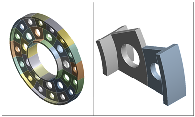
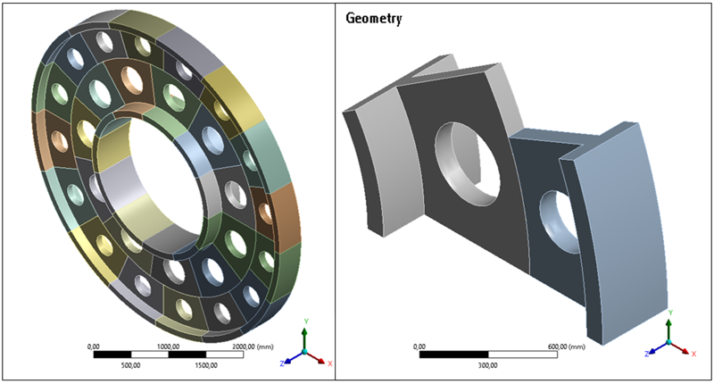
The model to be analyzed consists of a 2-stage disk with two series of stress relief holes located respectively on the inner and outer radius of the disk. The inner stage has 11 sectors and the outer stage has 16 sectors, as illustrated in the figure below. A rotational speed is applied to the whole structure, and the inner ring is fixed.
- Project Schematic in Workbench
Download the workbench project archive file (625 KB) for this tutorial here.
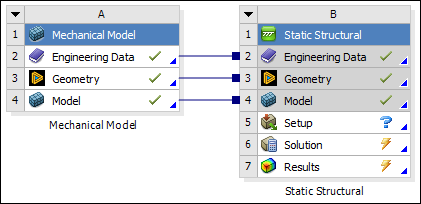
Browse to open the file Multi-HarmonicTutorial.wbpz, and observe the Project Schematic shown below in Workbench.
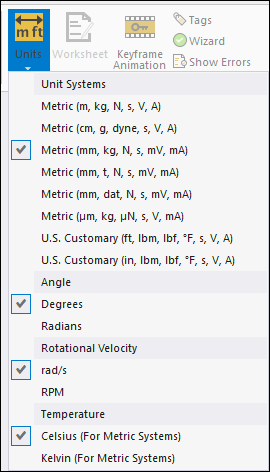
Double-click the Model (B4) cell to open Mechanical. From the Home tab in the application, verify that the unit system is set to Metric (mm, t, N, s, mV, mA).
Define a symmetry region for each stage using the Cyclic Region object.
Right-click the Model object and select .
Right-click Symmetry and select and specify its details as described in the following steps.
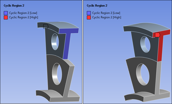
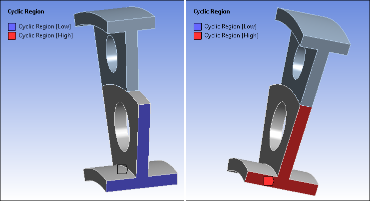
Select the face on the side of the first stage for the low boundary as illustrated in blue in the image below and click next to Low Boundary.
Select the face on the opposite side of the sector for the high boundary as illustrated in red in the image below and click next to High Boundary.
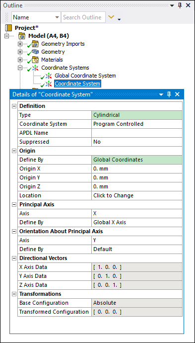
Set Coordinate System to the previously created cylindrical system.
Note: Since the order of the high and low boundaries does not have any impact on the solution, the red and blue selections in the above figure could be interchanged.
Using the above steps, create another Cyclic Region on the outer body, scoped as shown below.
Define each stage using the Stage object. A Stage includes all necessary meshes and boundary conditions to model a single cyclically symmetric structure which will be tied to another cyclically symmetric structure in a multistage cyclic symmetry analysis. To define the stages:
Right-click Symmetry and select and specify its details as described in the following steps.
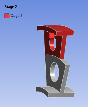
Scope the body illustrated below to specify the stage.
Set the Cyclic Region property to .
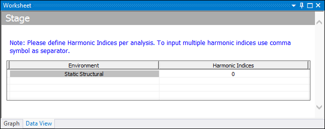
Note that the Harmonic Index is defined using the default, 0.
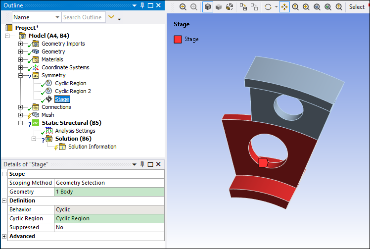
Using the above steps, create a second stage on the outer body as illustrated bellow.
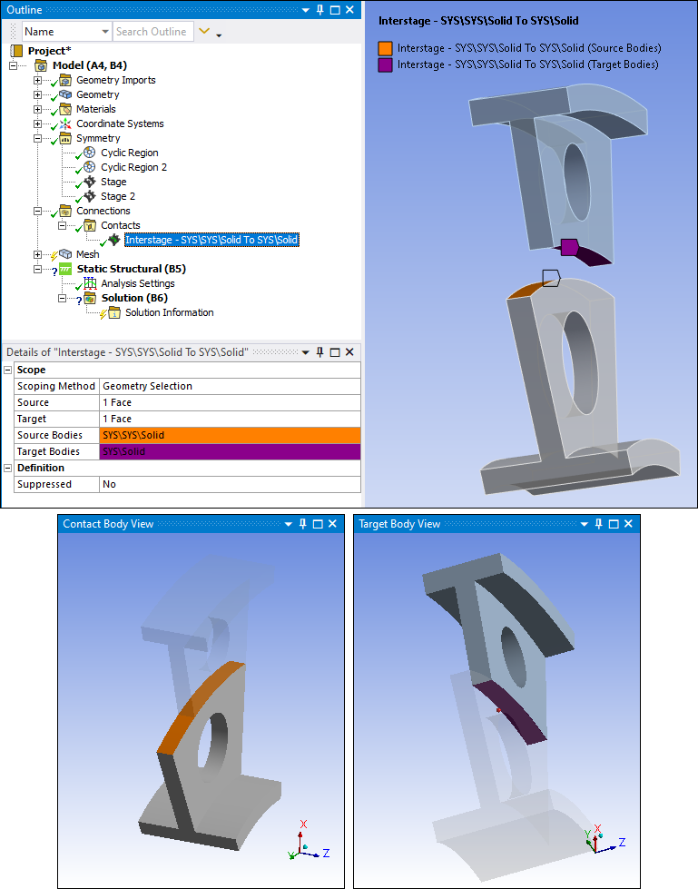
Define the connection between the contact region of different stages using an Interstage object. In a multistage analysis, a specific type of connection between the contact region of two different stages is defined using an Interstage object. Interstage connections are only valid for solid elements with degrees of freedom UX, UY, UZ or UX, UY, UZ, ROTX, ROTY, ROTZ.
To define the interstage connection:
First, you need to remove the automatically generated contact. Under the Connections object, right-click the Contacts object and select .
Right-click Connections, select .
Set the property by selecting the face of the first stage that will be in contact with the face of the second stage as indicated by the orange region in the figure below.
Set the property by selecting the contact face of the second stage, shown in purple in the figure below.
Note: Points c and d above are the Mechanical APDL recommendations for defining the interstage connection correctly, but the order is not important when using the Mechanical Application since it automatically inverts and if they are input in the opposite order.
Tip: Faces within the internal structure of the model must first be exposed so that you can select and scope them to the source or target properties of the interstage object. You can expose faces within the structure in one of two ways:
Use the Explode feature to create an imaginary distance between geometry bodies in the geometry view as seen in the figure above.
Hide the body that is obstructing the face: select the body, right-click in the geometry window, and select Hide Body (keyboard shortcut F9). To view all bodies again after selecting the face, right-click in the geometry window and select .
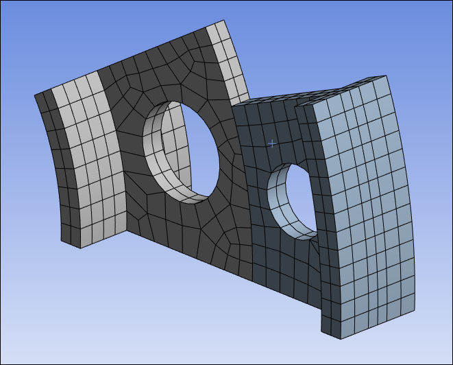
Select the Mesh object, right-click, and select . Note that the mesh of the contact region interfaces has quadratic elements of the same type and approximately the same size, as seen in the following figure.
- Specify Boundary Conditions
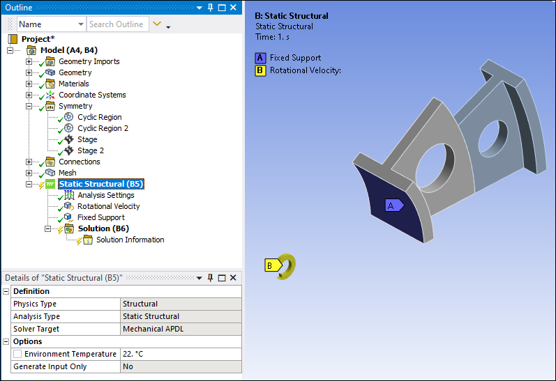
In this analysis, a fixed support is applied on the inner ring of the disc, and the entire structure is subjected to a rotational speed of 100 rad/s around the axis of symmetry. To apply a fixed support on the inner ring of the disc:
Right-click the Static Structural (B5) object and select .
Scope the inner ring of the disk (labeled A in the figure below) to the Geometry property of the fixed support object.
To apply a rotational speed of 100 rad/s around the axis of symmetry to the entire structure:
Right-click the Static Structural (B5) object and select . The Rotation Velocity boundary condition is automatically scoped to .
Set Define By to Components (required for cyclic symmetry).
Set Coordinate System to the cylindrical one you created previously.
Set the speed to 100 rad/s on the Z Component.
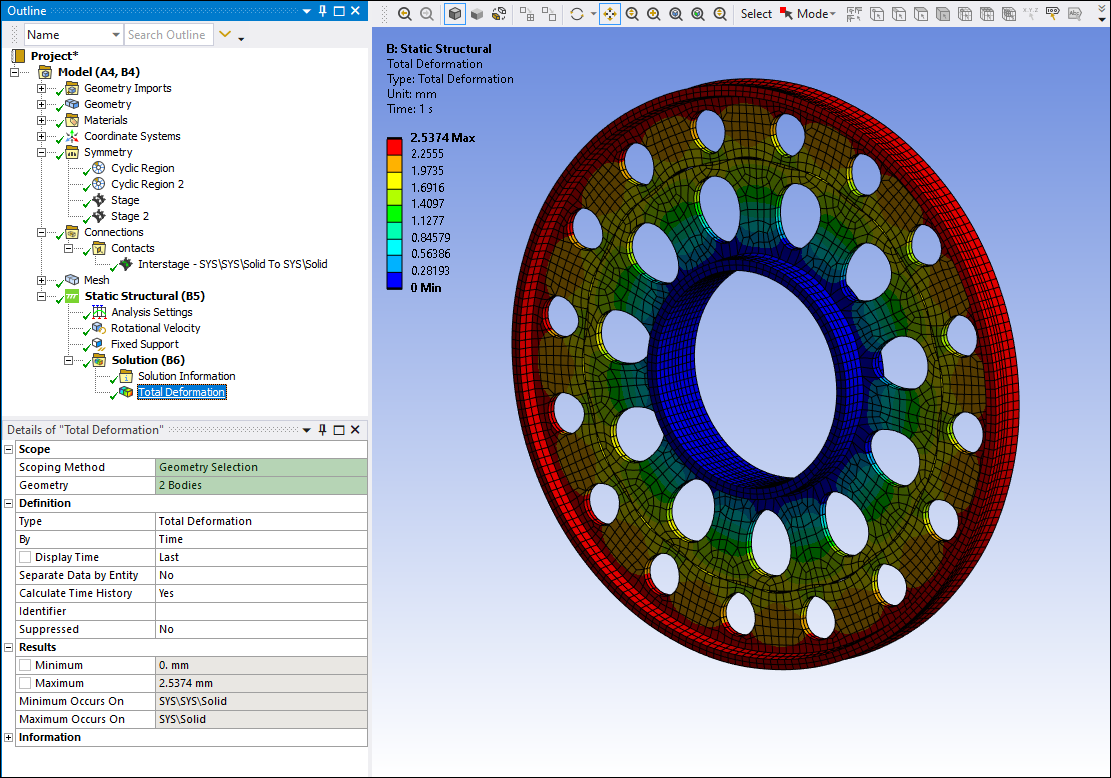
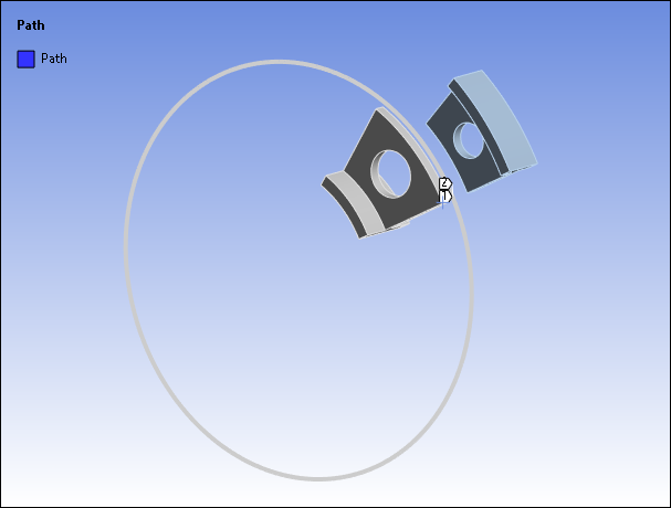
As detailed in the previous tutorial, Static and Modal Analysis of a Compressor Model with 4 Axial Stages, you can view the full structure in 360 degrees by setting the to 0 in solution details and using the option during postprocessing. This also enables you to visualize the results around an edge. This is useful to analyze displacement, verify the continuity of the interstage connection, and evaluate the presence of multiharmonic phenomena.
Right-click the Solution object and select . In its Details pane, select both bodies of the model in the geometry view, click in the Geometry property field.
Solve the analysis.
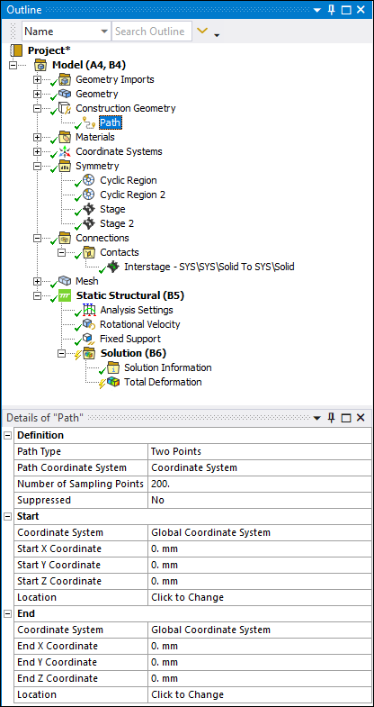
Now, we're going to use a Path as the scoping for this result. Select the Model object, open the Construction Geometry drop-down menu on the Model toolbar ribbon, and select Path. The the properties as follows:
Use the default setting for the Path Type property: .
Set the Number of Sampling Points property to
200.Set the Path Coordinate System property to the previously created cylindrical coordinate system.
Use the default setting for the Coordinate System properties of the Start and End categories: . The object should appears as shown below.
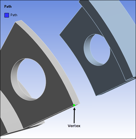
Scope the Location properties of the Start and End categories to the vertex highlighted below.
This scoping creates a circular path.
Insert another Total Deformation result and:
Set the Scoping Method property to .
Set the property to (created above).
Specify the Geometry property using the first stage body.
Solve the analysis.
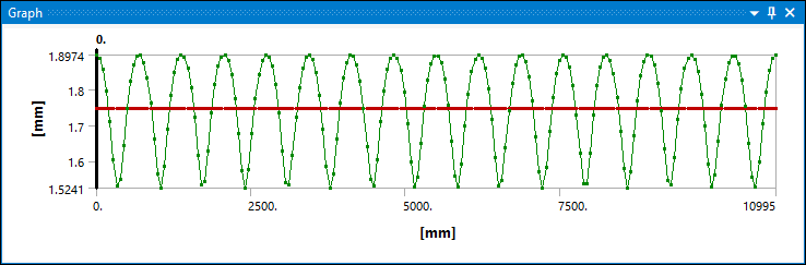
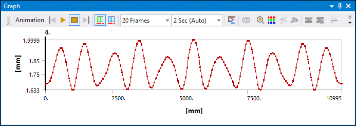
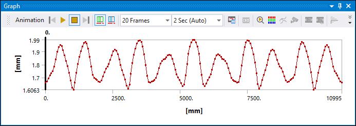
As illustrated below, the result shows the selected path 360° around the symmetry axis.
At this point, create another Total Deformation result, set the Path property to Path, and specify the Geometry property using the second stage (outer) body. Retrieve the result for the Total Deformation, as shown below.
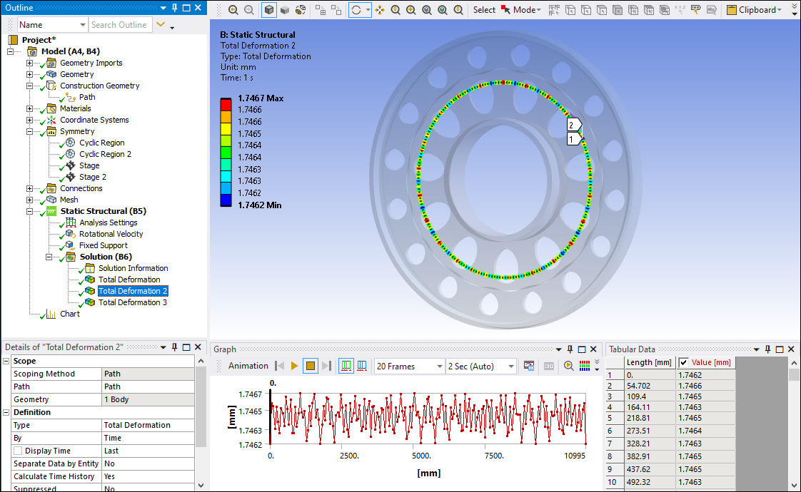
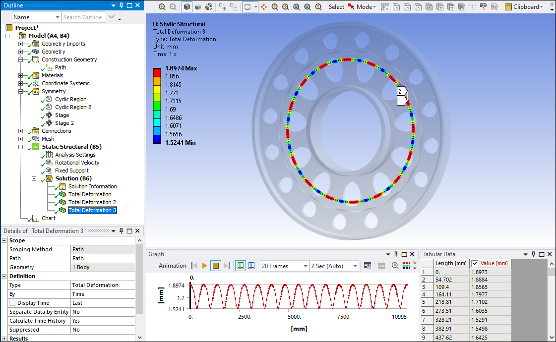
The content of the Graph and Tabular Data windows relate the values of each point to its position along the path. The deformations of each path have different values, which indicates a discontinuity in the contact interface. To investigate this, create a Chart object to plot the two total deformations.
To chart deformations on the interstage interface between stages to analyze continuity:
Select the two Total Deformations created using paths and select the Chart option on the Home tab to insert a chart object that overlays the curves presented in results.
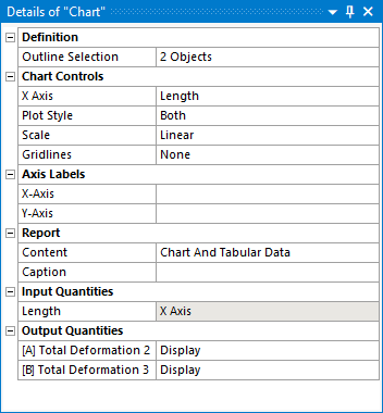
This chart enables an analysis of the continuity between the edges.
Note that there is a discontinuity between the stages in the contact interface because displacements at the interstage boundary are not matching between the inner and outer stage. This indicates that some harmonics may be missing in the response calculation that are required to accurately simulate the true response of the structure. To investigate further this discontinuity problem and improve accuracy, it is necessary to add more harmonics in the analysis.
Due to the multiharmonic phenomenon, it is clear that the interstage displacement is a composition of several harmonic functions. In the previous analysis, only the HI = 0 harmonic was considered for each stage.
Performing an analysis considering all harmonics present in each stage would increase the time and computational effort enough to defeat the purpose of multistage modelling. It is therefore necessary to choose beforehand the minimum set of harmonic indices required to compute the correct response. This can be accomplished by determining which harmonics are activated in each stage and evaluating their relevance in the solution, since some act more significantly than others.
Note: Randomly choosing harmonic indices could lead to a solver error if the chosen HIs are uncoupled, resulting in no constraint equations generated between stages. Follow the procedure outlined here to choose which HIs to include in your analysis.
One way to determine which HIs to use at each stage is to evaluate the relationship
between the nodal diameters and HIs. The number of HIs in a stage is defined by the number of
sectors (N) into which the 360-degree model was divided. The maximum harmonic indices (HI) in
a stage is defined as: 
The following equation describes the relationship between the different nodal diameters
d and harmonic indices of a cyclic structure:
where m is an integer.
- Example
For a model with two stages having 6 and 12 sectors, respectively, the relationship between HI and d from the above equations is:
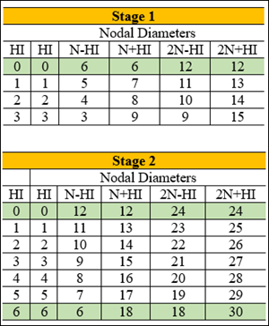
The tables show clearly that considering only HI = 0 for stage 1 and 2 will lead to incomplete coupling between the stages (nodal diameters 6, 18, 30, etc. will be missing for stage 2). It is necessary to combine the harmonics 0 and 6 of stage 2 to obtain HI 0 in stage 1.
To reduce the discontinuity in this example case, the combined response of harmonics 0 and 6 from stage 2 must be used with HI = 0 in stage 1.
The analysis is simplified if the sector counts between the stages has the same common divisors. In this example, the different harmonics for the stages can share the same nodal diameters number. The analysis described above is also valid for cases that do not have a common divisor and for models with more than two stages.
Note: The Multi-stage Harmonic Choice Wizard calculates and lists relevant harmonic indices based on the equations above to facilitate HI selection. For more information, see Multistage Harmonic Choice Wizard.
- Multiharmonic Model
The model analyzed in this tutorial has 11 sectors in the inner stage and 16 in the outer stage. Analyzing the nodal diameters results in the following:
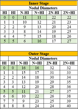
In this case, it is a little more difficult to identify the complementary harmonics indices of each.
Combining HI 0 and 5 in the inner stage with HI 0 and 5 in the outer stage is a good first step. Since a large part of the nodal diameters corresponds to these harmonic indices, a preliminary analysis can check if considering only these harmonics is sufficient or if it is necessary to add more. Since lower numbered nodal diameters influence the response more significantly, the coupled nodal diameter of the first columns should be primarily chosen.
Mechanical APDL commands must be used to perform the multiharmonic static analysis since the Mechanical Application does not yet support it.
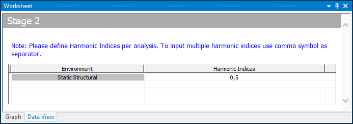
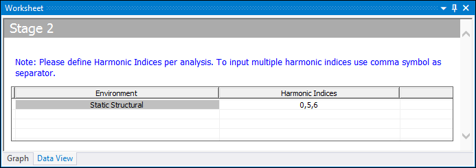
- Harmonic Indices
To add more harmonics to the solution, you must modify the harmonic Indices definition in the Worksheet pane for each stage.
The loading is applied only in the base and duplicate sector of the HI=0 stage. The rotational speed must be defined using the Mechanical APDL CMOMEGA command. To start the analysis:
Right-click the Rotational Velocity boundary condition and select .
Right-click Static Structural (B5) select > .
In the Commands (APDL) object, copy and paste the following command content. For more information about the commands used in this tutorial, consult the Multistage Cyclic Symmetry Analysis Guide and the Mechanical APDL Command Reference.
Stage_1 = '_STAGE$$'    ! change the inner stage name (replace $$ by proper number).
Stage_2 = '_STAGE££'                 ! change the outer stage name (replace ££ by proper number).
csys,12
cmsel,s,%Stage_1%_0_BASE_ELM                ! apply loading to HI=0 clones only
cmsel,a,%Stage_1%_0_DUPL_ELM
cmsel,a,%Stage_2%_0_BASE_ELM
cmsel,a,%Stage_2%_0_DUPL_ELM
cm, Selection,ELEM
cmomega,Selection,,,100
ALLSEL
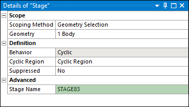
Make sure that you change the stage name in the command entry. This value is available from the Details of the Stage objects has shown below.
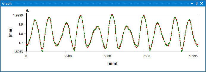
These images show that the curves have similar shapes and close peak values.
A comparison of the two curves overlapping is shown using the Chart object. This shows that the continuity of the model has improved considerably by adding the harmonic indices.

If you want to further improve the continuity of the model, try adding HI = 1 in the first stage and HI = 6 in the second.

Congratulations! You have completed the tutorial.