


This example demonstrates the use of multistage cyclic symmetry analysis to examine the behavior of a compressor model with four axially aligned stages.
| Analysis Type | Static and Modal Analysis |
| Features Demonstrated | Static, modal, and prestressed modal multistage cyclic symmetry analysis, loads, harmonic index of an analysis |
| Licenses Required | Ansys Mechanical Enterprise/Enterprise Solver/Enterprise PrepPost |
| Help Resources | Multistage Cyclic Symmetry Analysis Guide |
| Tutorial Files | MultistageTutorial.wbpz |
This tutorial guides you through the following topics:
Multistage cyclic symmetry analysis provides a way to combine two or more independent cyclically symmetric systems with different sector counts while still leveraging the efficiency of the cyclic symmetry procedure. The procedure described in this tutorial can be used for any system that has one or more cyclically symmetric physical structures.
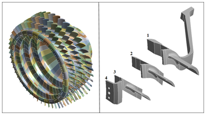
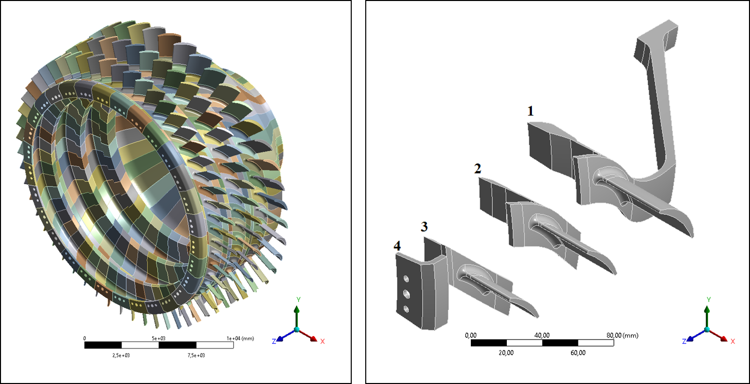
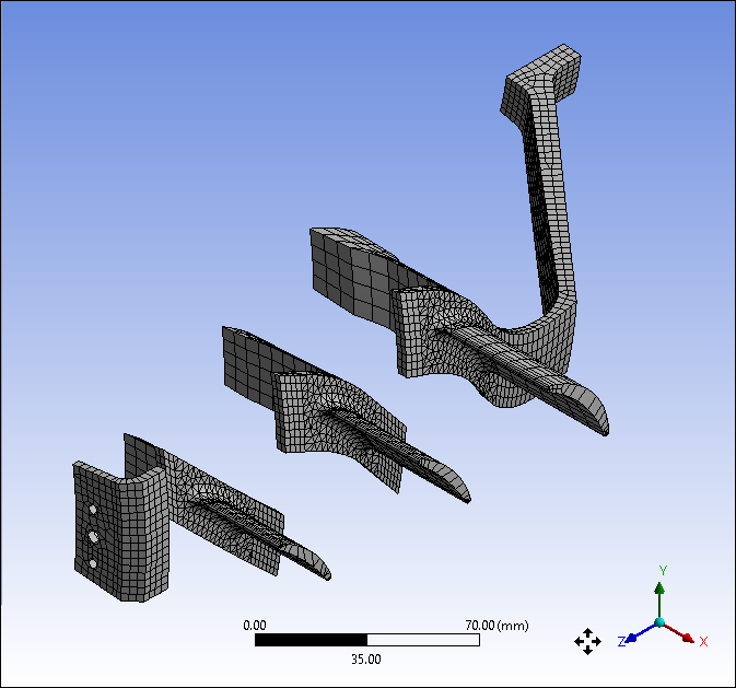
The Compressor Model to be analyzed consists of three blade rows and a rim that can be simplified as a multistage system with four axially aligned cyclic stages merged at three interstage boundaries as shown in the figure below. The model is fixed along the rim. It has a rotational speed, and the blades are subjected to pressure and temperature variations along the stages due to air compression. Multistage cyclic symmetry analysis is used to determine the deformation of the structure due to the imposed load and to determine the natural frequencies of the structure. For this, a static, modal and pre-stressed modal analysis will be performed.
The stages have the following sector counts:
Download the workbench project archive file (59 MB) for this tutorial here.
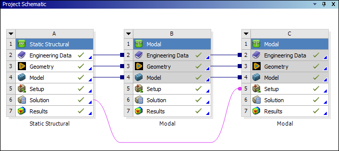
Browse to open the file MultistageTutorial.wbpz, and observe the Project Schematic shown below in Workbench.
Double-click the Model (A4) cell to open the Mechanical Application.
Define the multistage model
This section describes how to specify the multistage cyclic symmetry objects for the four-stage model and prepare other general aspects of modeling in the Mechanical Application. The steps to set up the multistage model are as follows:
either a Cyclic Region or Pre-Meshed Cyclic Region object to define the symmetric region,
a Stage object to specify the bodies in a given cyclic component, and
an Interstage object to specify the connections between each Stage.
The Cyclic Region and Pre-Meshed Cyclic Region objects require selection of the sector boundaries, together with a cylindrical coordinate system whose Z axis is collinear with the axis of symmetry, and whose Y axis distinguishes the low and high boundaries. This tutorial uses the cyclic region object to define symmetry regions.
In the Pre-Meshed Cyclic Region, the low/high edge nodes should preferably match, but if not, they will be mapped automatically. Automatic mapping will result in a decrease in the accuracy of the results.
Use the Stage object to define the bodies present in the model that correspond to a given cyclic component and the Interstage object to specify the connections between each stage of the multistage analysis.
Note: Multistage cyclic symmetry can be used to model one or more cyclic stages in combination. You can combine up to 100 stages with each stage having up to 360 sectors. For more information about the features and limitations of this tool, see Multistage Cyclic Symmetry Analysis in the Mechanical User's Guide and Multistage Cyclic Symmetry Analysis Guide in the Multistage Cyclic Symmetry Analysis Guide
Define a cylindrical coordinate system
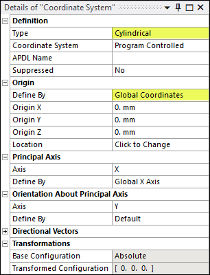
Right-click the Coordinate Systems object in the Outline window and select . In the Details view, set the Type property to and the Define By property to as highlighted in the following figure.
The axis of symmetry does not need to be aligned with the global CS axis.
Define the symmetry region using the cyclic region object
Right-click the Model object and select .
Right-click Symmetry and select and specify its details as described in the following steps.
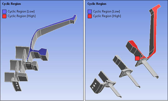
Select the four faces on one side of the first stage for the low boundary as illustrated in blue in the image below and click next to Low Boundary.
Select the four matching faces on the opposite end of the sector for the high boundary as illustrated in red in the image below and click next to High Boundary.
Set Coordinate System to the previously created cylindrical CS.
Note: Since the order of the high and low boundaries does not have any impact on the solution, the red and blue selections in the above figure can be interchanged.
Steps ii through v above define the cyclic region for stage 1. Repeat these steps three more times to define cyclic regions for the remaining stages (stage 2, 3, and 4 in Figure 14.1: Multistage Model of the Compressor).
Define the stages
A stage includes all necessary meshes and boundary conditions to model a single cyclically symmetric structure which will be tied to another cyclically symmetric structure in a multistage cyclic symmetry analysis.
To define the stages:
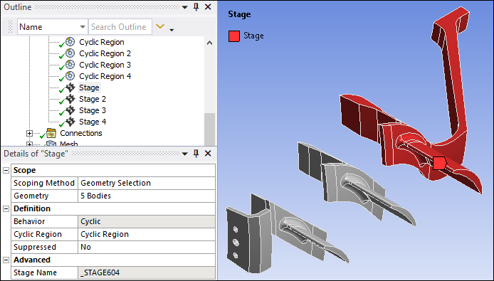
Right-click Symmetry and select and specify its details as described in the following steps.
In Geometry, select all bodies that make up the stage, as shown in the figure below.
In the Cyclic Region property, specify the corresponding to your body selections.
Steps i through iii above define stage 1. Repeat these steps three more times to define the remaining stages (stage 2, 3, and 4 in Perform the Modal Analysis).
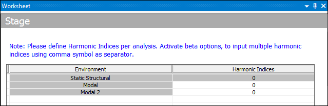
When you select a stage object, the stage worksheet displays automatically (see the screenshot below). This Worksheet is used to specify the Harmonic Index values for all analyses in the model. For a static analysis, the Harmonic Index is set to zero by default.
More information about Harmonic Indices and steps to take to change the HI will be presented in the section describing the modal analysis. For a tutorial on how to use Beta options to include multiple HIs in a single analysis, see Static Analysis of a 2-Stage Disk with Pinholes.
Define interstage connections
In a multistage analysis, a specific type of connection between the contact region of two different stages is defined using an Interstage object. Interstage connections are only valid for solid elements with degrees of freedom UX, UY, UZ or UX, UY, UZ, ROTX, ROTY, ROTZ.
To Define the interstage connections:
Under Connections, if contacts exist, right-click Contacts and select to remove the automatically generated contacts.
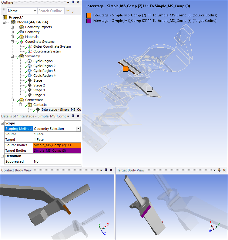
Right-click Connections, select and specify its properties in the details window as described in the following steps.
Set the property by selecting the face of the first stage that will be in contact with the face of the next stage as indicated by the orange region in the figure below.
Set the property by selecting the contact face of the next stage, shown in purple in the figure below.
Note: Points iii and iv above are the Mechanical APDL recommendations for defining the interstage connection correctly, but the order is not important when using the Mechanical Application since it automatically inverts and if they are input in the opposite order.
Right-click Contacts, select and select and scope the appropriate faces to the source and target properties of the next interstage connection.
Repeat the previous step to create the last interstage connection.
Tip: For geometries in which the faces of the Interstage regions are in contact, there is a faster way of defining the connections:
Right-click Connections and select
Right-click Connections Group and select
Note that this automatic creation of the Interstage connections only works if the stage objects are previously defined. You can use feature to create the interstage connection between stage 3 and stage 4 without having to manually select the target and source faces.
Mesh the model
It is recommended that the Interstage region meshes have quadratic elements of the same type and approximately the same size. This improves the accuracy of the results of a multistage cyclic symmetry analysis.
The meshes of the Interstage regions do not have to be adjacent to each other in the circumferential direction, and the sectors of each stage can start at different locations along the circle of symmetry as illustrated in the following figure.
Analysis Settings
In Static Structural Analysis Settings, set Large Deflection to ON.
Boundary Conditions
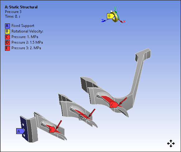
For this analysis, the following boundary conditions must be specified:
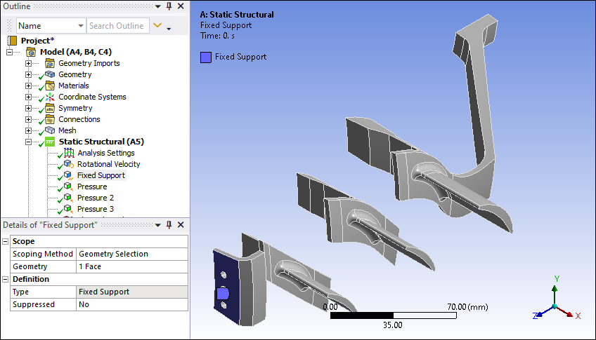
The compressor is fixed on one side.
It has a rotational speed of 1000 rad/s around the axis of symmetry.
Right-click the object, select , and specify its properties in the details window as described in the following steps.
Set Define By to Components (required for cyclic symmetry).
Set Coordinate System to the cylindrical one you created previously.
Set the speed to 1000 rad/s on the Z Component.
Its pressure and temperature increase along the stages due to fluid compression.
For stages 1, 2, and 3 in Figure 14.1: Multistage Model of the Compressor, insert three Pressure objects, scope them to the faces of the blades at each stage, and set the magnitude to a value of 1, 1.5, and 2 MPa, respectively.
For each of the four stages, right-click the object, select , scope it to all the bodies in the stage, and set the magnitude in the details view to the following values: 200, 250, 300 and 350 °C.
Note: There are some limitations and restrictions on loads applied in the multistage analysis. The most important ones are:
No user-defined constraints should be applied at the cyclic or interstage boundaries.
No contact or joints can be used at the cyclic or interstage boundaries. This includes remote loads that touch these boundaries, which are applied using a pilot node.
Loads are not permitted at the interstage boundaries.
All loads are based on HI = 0 and are axisymmetric.
Solution (A6)
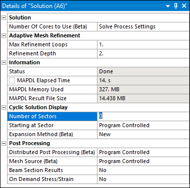
It is possible to define the number of sectors that you want to show in the solution by changing the Number at Sectors in the solution details. This number is applied in all stages of the model. If you do not change the default settings, it will show the first stage of each sector.
To view the full 360 degrees model, change the Number of Sectors to the default value of 0 to use the Program Controlled option.
Solve the model
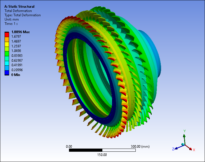
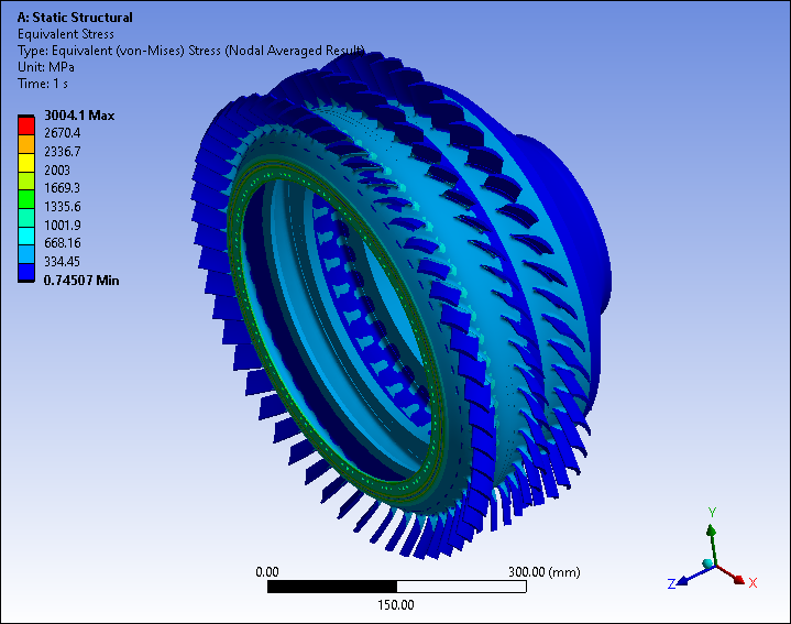
Insert a Total Deformation and Equivalent Stress and solve the model. If the model has an error during the solution, try right-clicking and solve the model again. The expanded analysis results are shown below:
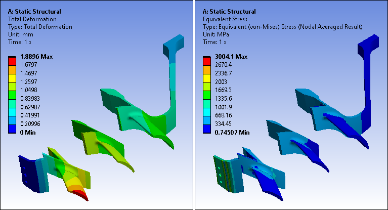
To view the results of a single sector, set the Number of Sectors set to 1 in the solution details window, and solve. The single sector results are shown below.
A modal analysis is used to determine the vibration characteristics (natural frequencies and mode shapes) of the structure.
In this analysis, the natural frequencies of the structure are determined without considering the loading. To set up the Modal Analysis, apply the fixed support boundary condition and solve:
Right-click the Modal (B5) object and select .
In the Geometry property, choose the outer face of the rim, as shown in Figure 14.9: Fixed Support.
Right-click the Solution (B6)object and select solve.
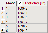
The first six HI = 0 frequencies found for this model are listed in the figure below.
As in the previous analysis, it is possible to choose the number of sectors presented in the result in the solution details window.
In a multistage modal analysis, it is important to carefully choose the set of harmonic indices associated with the solution. Because all stages have a different number of sectors, the physical solution contained in each harmonic index (HI) is different. The underlying assumption for multistage cyclic analysis is that the main coupling between stages appears between the same harmonic indices.
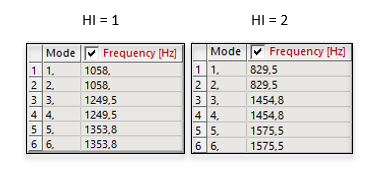
To modify the HI of the solution, it is necessary to change the HI used in each stage. To do this, click the Stage object, input the desired HI in the stage object worksheet (shown in Figure 14.6: Stage Worksheet), and run the solution again. For cases where all stages of the system vibrate at HI = 1 and 2 respectively, the following frequencies are calculated.
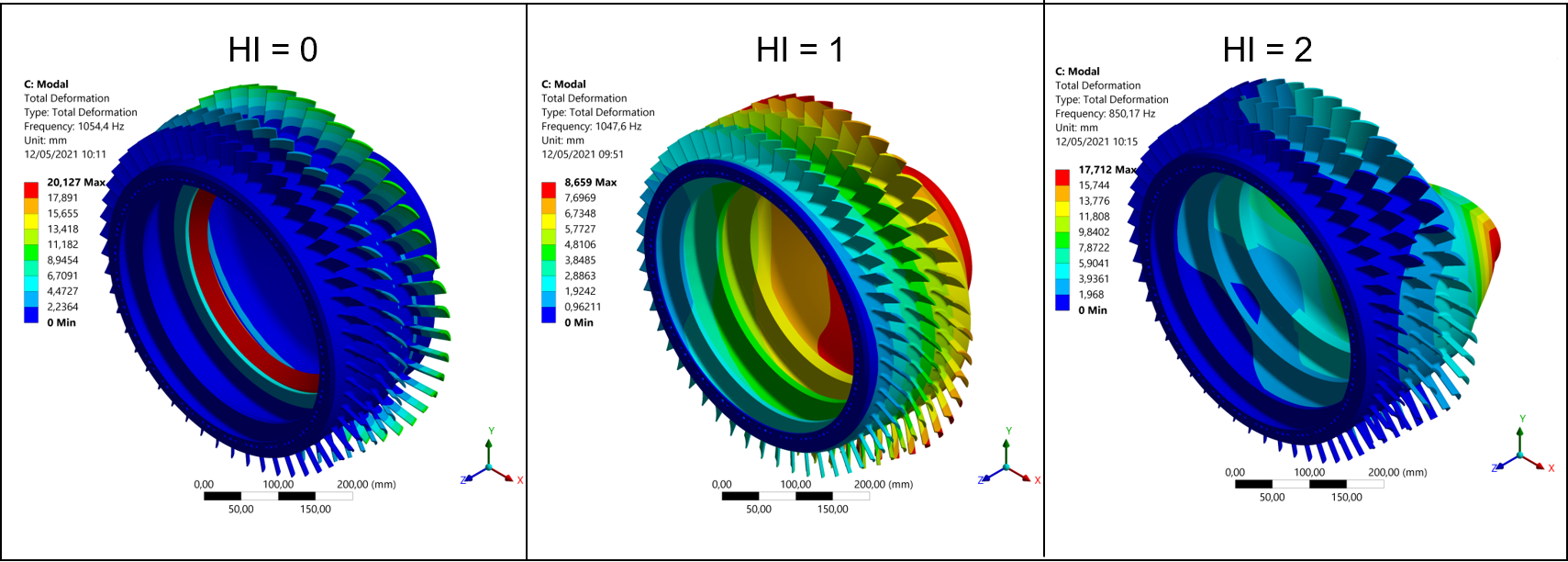
The mode shapes found for the first frequency of each HI analyzed are shown below.
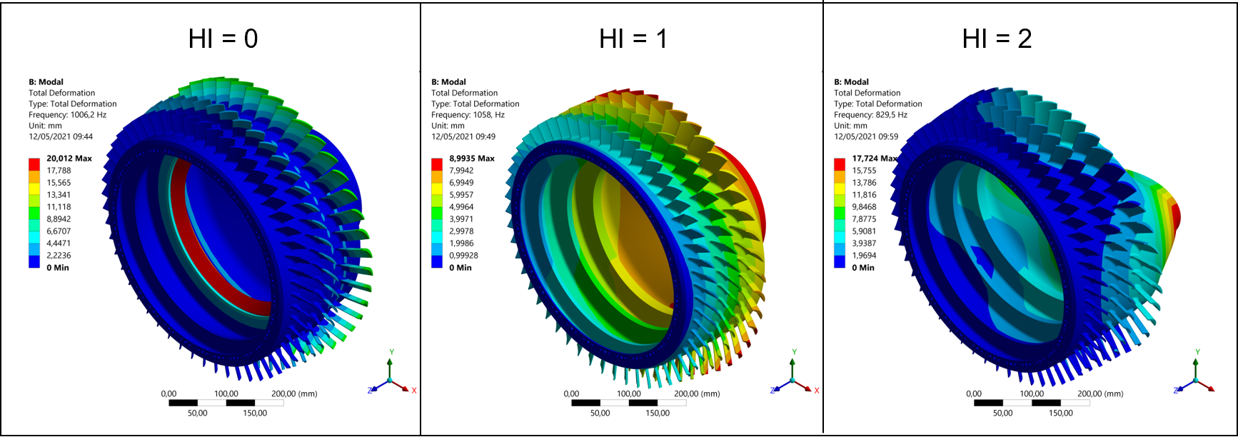
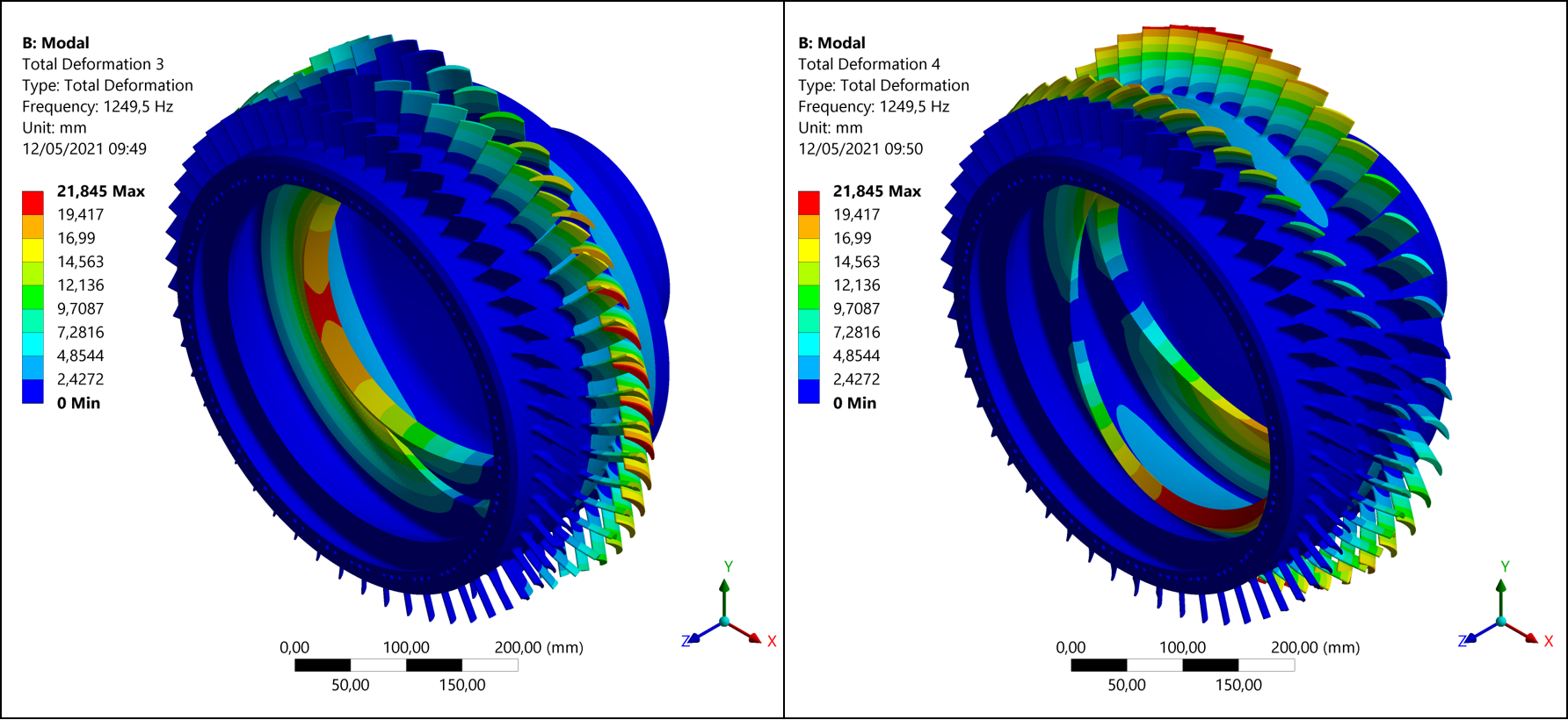
Note that for HI > 0, the frequencies appear in pairs as expected due to cyclic symmetry (Figure 14.16: Frequencies for HI = 1 and HI = 2). The difference between the two modes at the same frequency is the direction in which the deformation occurs. Mode shapes 3 and 4 for HI = 1 are shown below.
Pre-Stressed Modal Analysis
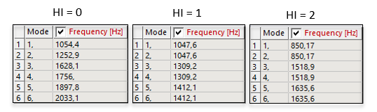
On the Modal 2 (C5) > Pre-stress environment choose Static Structural and click Solve. The analysis results for HI = 0, 1, and 2 are shown below.
The mode shapes found for the first frequency of each HI analyzed are shown below.
Congratulations! You have completed the tutorial.