


In this tutorial, you will perform a fatigue analysis of a simple shaft under combined bending and torsion using the Mechanical DesignLife Add-on. The example uses linear stresses from two load steps in a Mechanical simulation, and combines them with two measured non-proportional load histories.
| Analysis Type | Fatigue |
| Features Demonstrated | DesignLife Add-on, DesignLife system, analysis settings for fatigue calculation, inputs and loading conditions |
| Licenses Required | Ansys Mechanical Enterprise PrepPost and Ansys nCode Premium/Enterprise |
| Help Resources | DesignLife Add-on |
| Tutorial Files | FatigueShaft.zip |
This tutorial guides you through the following topics:
Data files for this tutorial can be found here on the Ansys customer site.
The files you need are:
sae_shaft_1_Addon.wbpz - this is the input model that you will set up during the steps defined below. Copy this file to a working folder and complete the worked example using the copy.
sae_shaft_1_Addon_completed.wbpz - this is an example of the completed model once all the steps have been followed.
Start Workbench, and select > .
Browse to the working folder and select sae_shaft_1_Addon.wbpz.
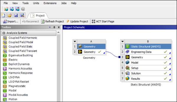
This Workbench project contains the Static Structural system.
Double click the Results cell to open Mechanical.
To make the DesignLife capabilities available, click the icon in the ribbon.
The icon is highlighted in blue, indicating that the add-on is loaded.
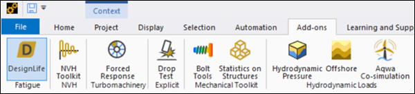
Once the add-on is loaded, the Ansys nCode DesignLife ribbon is visible, exposing all the DesignLife capabilities.
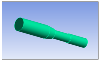
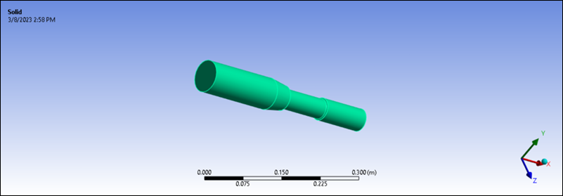
The model consists of a single part, named Solid.
Expand the geometry list, select the Solid part, and verify in the Details window for Solid that the Material Assignment is
Carbon Steel SAE1045_450_QT.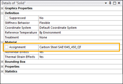
Note:
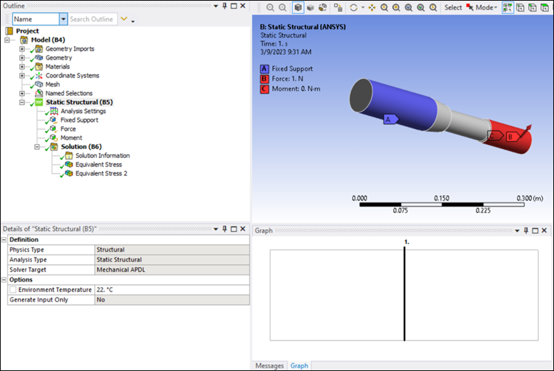
Carbon Steel SAE1045_450_QTis available as part of the ncode material library. This can be found in the Ansys nCode DesignLife installation under GlyphWorks\mats\nCode_matml.xml.The model contains a single analysis with two load steps. The left end of the shaft is fully fixed, and the right end has two loads defined. The first load is a force applied in the global Y direction, with a magnitude of 1 N at time 1 s, and a magnitude of 0 N at time 2 s.
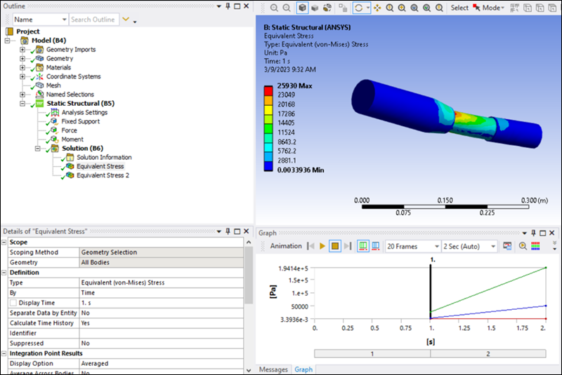
The resulting Equivalent Stress (von Mises) state is displayed, and shows a classic bending stress distribution concentrated around the shoulder radius of the shaft.
The second load is a torque applied in the global X direction, with a magnitude of 0 Nmm at time 1 s, and a magnitude of 1000 Nmm at time 2 s.
The resulting stress state from the torque loading is shown below.
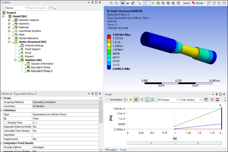
The structural analysis is completed and has stress results available for DesignLife.
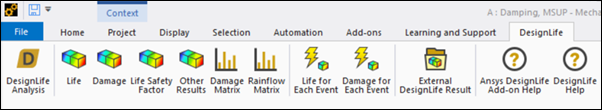
From the DesignLife toolbar, select to insert a new DesignLife analysis directly from Mechanical.
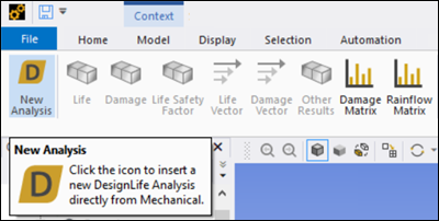
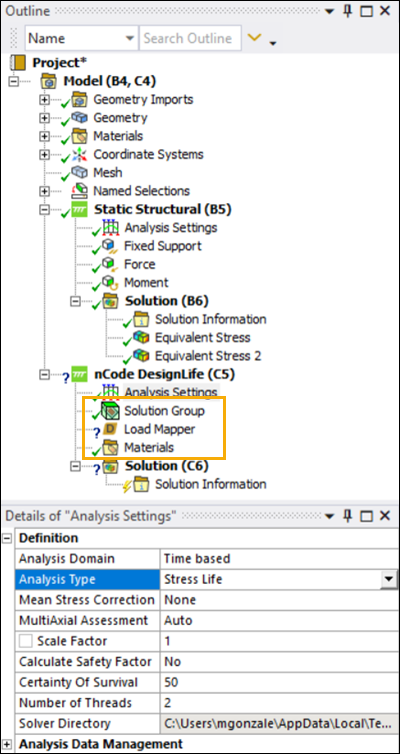
Click the DesignLife Analysis icon and verify that the nCode DesignLife (C5) object is inserted into Mechanical.
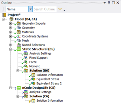
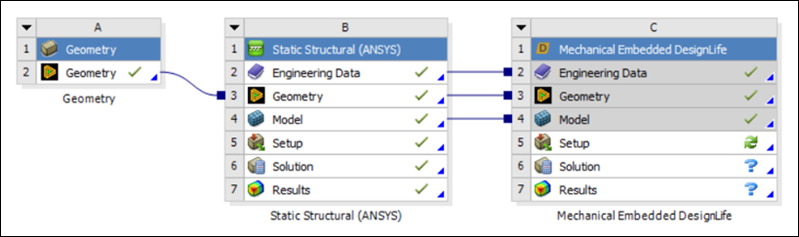
If you return to the Project schematic in Workbench, the system is also visible connected to the Static Structural system. The Mechanical Embedded DesignLife system is incorporated into the schematic, sharing Engineering Data, Geometry and Model cells with the Mechanical system.
For this example, you will perform a fatigue calculation using Time Series loading. The Analysis Domain defaults to the option when the DesignLife system is connected to a Static Structural system.
Set the Analysis Type to . The main objects required for a DesignLife analysis are then generated automatically. These are the Solution Group, Load Mapper and Materials objects.
Defining inputs and loading conditions
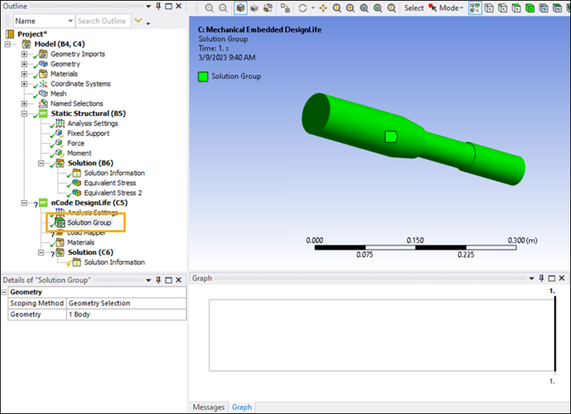
The Solution Group defines the portion of the geometry that will be calculated for the fatigue analysis. By default, all bodies are selected. In this case, there is only one geometry, so there is no need to modify the setting.
The fatigue loads can be either Constant Amplitude, Time Step or Time Series for the Time based domain.
Select the Load Mapper and click the button under Add Loading Event. This adds the first Loading Event.
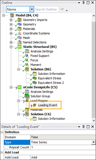
Note: Loading Events in the Analysis Domain can include multiple loadings of the same type. The Time Series loading reads a time series data file from disk.
If any of the time series test list are schedules, or any files have a Repeat Count other than 1, then a Repeat Count is written to the metadata for each test output. Repeat counts can also be added to each test set to define a schedule.
Define the loading events
Loading Event 1
Set the Repeat Count to
1000and set the following options for the Time Series Load in Loading Event 1:Environment: This selects the system from which the .rst file, which will be picked for the nCode fatigue analysis. Select the environment so that the results of the static system system are picked.
Define By: The loading can be defined by time or step. In this case, pick the loading corresponding to
1.0s in the Static Structural system.Scale Factor: All the coefficients set in the input time series are multiplied by this factor. Set it to
8000.Static: You will not include static offset loading.
Input File Definition: When importing a time series file you have two ways of defining how the imported files are stored. If you want the file to be local to your machine, load it with the Input File Definition set to an . If you want the file to be contained within the project, load it as a . For this scenario, use .
Input File: Load the smallhistory.dat from the input files.
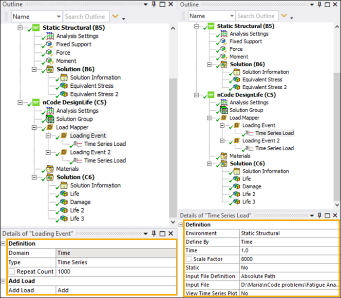
Loading Event 2
Set the Repeat Count to
5000and set the following options for the Time Series Load in Loading Event 2:Environment: Select the environment.
Define By: The loading can be defined by time or step. In this case, pick the loading corresponding to
2.0s in the Static Structural system.Scale Factor: Set to
2000.Static: You will not include static offset loading.
Input File Definition: Set to .
Input File: Load the smallhistory2.dat from the input files.
Right-click the Solution (C6) object in the project tree and select .
While solving, selecting Solution Information will show the solver's progress and display errors as they are encountered.
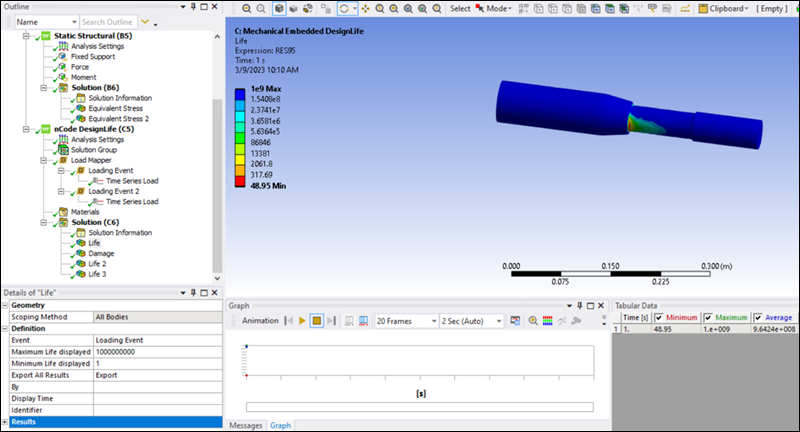
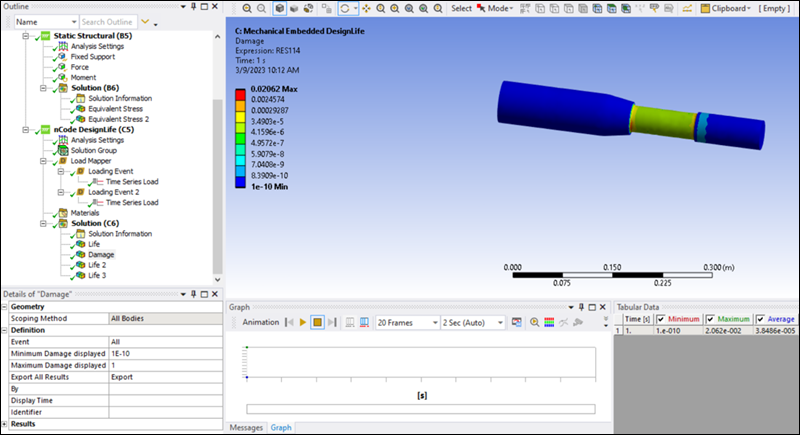
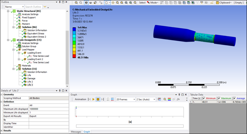
The fatigue results may be viewed as either life or damage. You can add a result by selecting the DesignLife toolbar with Solution active in the tree. Alternatively, right-click the Solution (C6) object and insert the following results:
Select > and scope to
Select >
Select > and scope to
Select >
Right-click the Solution (C6) object in the project tree and evaluate all the results (see below).
Life Result for Loading Event 1
Damage Results for all Loading Events
Life Result for Loading Event 2

Life Results for all Loading Events
You have completed the fatigue analysis and accomplished the overall objective for this tutorial.
Congratulations! You have completed the tutorial.