This chapter include several Material Processing Tutorials for Ansys Fluent.
The information in this chapter is divided into the following sections:
This tutorial is divided into the following sections:
This tutorial illustrates the simulation of a 3D extrusion process using the Fluent Materials Processing workspace (Fluent Materials Processing Workspace). The workspace will allow you to set up and solve a polymer extrusion problem so you can easily obtain an accurate prediction of the extrudate shape for a given die geometry under prescribed operating conditions.
In this tutorial you will learn how to use the Fluent Materials Processing workspace to:
Easily set up your extrusion simulation
Calculate a solution
Analyze the results.
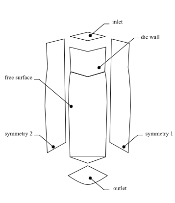
This problem deals with the flow of a Newtonian fluid through a three-dimensional die. Due to the symmetry of the problem (the cross-section of the die is a square), the computational domain is defined for a quarter of the geometry and two planes of symmetry are defined.
The melt enters the die as shown in Figure 3.1: Problem Description at a flow rate of Q = 10 cm3/s (a quarter of the actual flow rate) and the extrudate is obtained at the exit. At the end of the computational domain, it is assumed that the extrudate is fully deformed and that it will not deform any further. It is assumed that subdomain 2 is long enough to account for all the deformation of the extrudate.
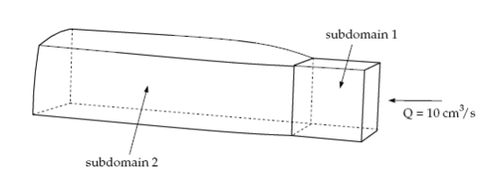
The incompressibility and momentum equations are solved over the computational domain. The domain for the problem is divided into two subdomains (as shown in Figure 3.1: Problem Description) so that the remeshing algorithm can be applied only to the portion of the mesh that will be deformed. The subdomain 1 represents the die where the fluid is confined. The subdomain 2 corresponds to the extrudate that is in contact with the air and can deform freely. The main aim of the calculation is to find the location of the free surface (the skin of the extrudate).
The boundary sets for the problem are shown in Figure 3.2: Boundary Sets for the Problem, and the conditions at the boundaries of the domains are as follows.
boundary 1: flow inlet, volumetric flow rate Q = 10 cm3/s
boundary 2: zero velocity
boundary 3: symmetry plane
boundary 4: symmetry plane
boundary 5: free surface
boundary 6: flow exit
The following sections describe the setup and solution steps for this tutorial:
To prepare for running this tutorial:
Prepare a working folder for your simulation.
Download the
3d_extrusion.zipfile here .Unzip the
3d_extrusion.zipfile you have downloaded to your working folder.The mesh file
ext3d.mshcan be found in the unzipped folder.
Use the Fluent Launcher to start Ansys Fluent.
Select Materials Processing in the list of Fluent workspaces.
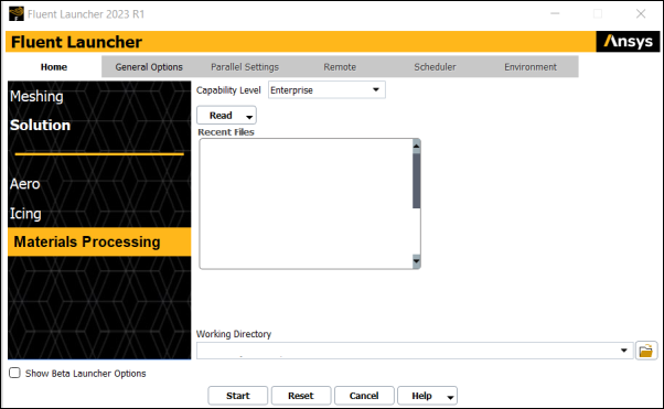
Click Start.
Clicking Start in the Fluent Launcher opens the Fluent Materials Processing workspace.
The workspace is a version of Ansys Fluent that utilizes the power of the Ansys Polyflow solver to simulate polymer flows such as extrusion, blow molding, pressing, and so forth.
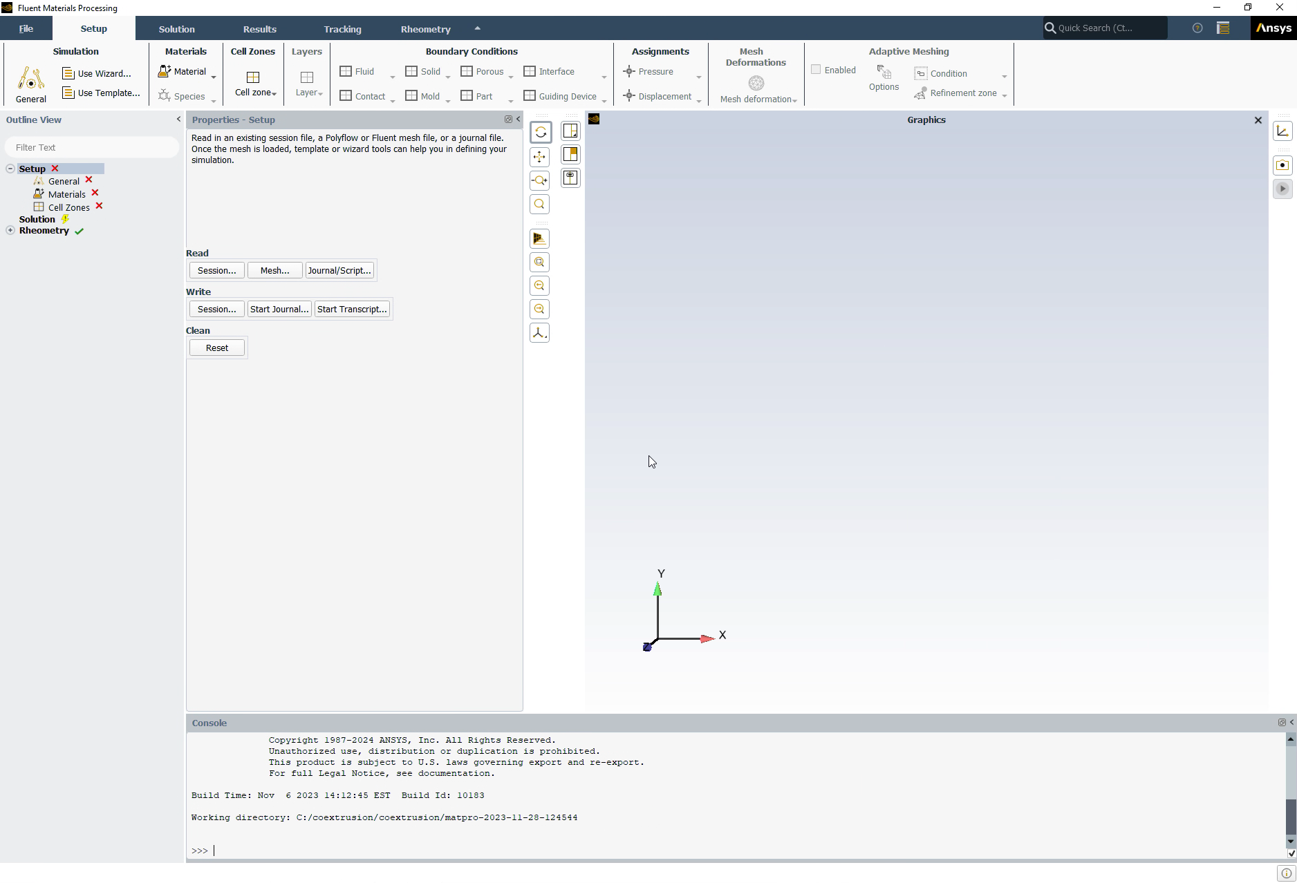
Open an extrusion geometry by reading in a Polyflow mesh file.
In the Setup properties, under Read, click the Mesh... button.
You can also use the File menu, and choose Read > Polyflow Mesh....
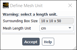
Locate and select the mesh file from your working folder (
ext3d.msh)Set the Mesh Length Unit to cm, and close the dialog box.
Set up an extrusion simulation (using the Simulation category of the Setup Ribbon).
 Setup
→ Simulation → Use
Template...
Setup
→ Simulation → Use
Template...
This will display the Simulation Template dialog.
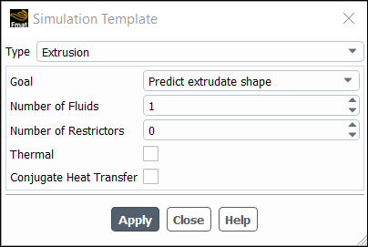
Set the Type to Extrusion.
Set the Goal to be Predict extrudate shape.
Keep the Number of fluids as 1.
Click Apply.
This will instruct the workspace to set up the appropriate objects and settings based on your selections.
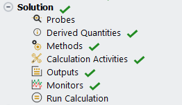
Note: Notice the Outline View's use of status icons. A green check mark indicates the properties of that object are satisfactory. A red 'x' indicates that attention is required for that object.
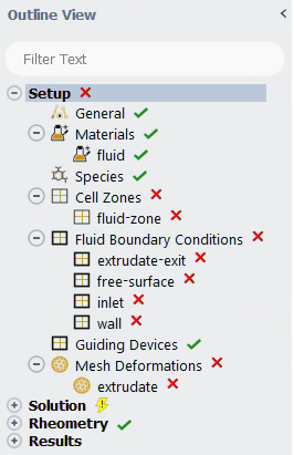
You can progress down the Outline View (or across the Ribbon) to complete your simulation settings using each object's property pages.
Click the General node in the Outline View to display general settings for the problem setup.
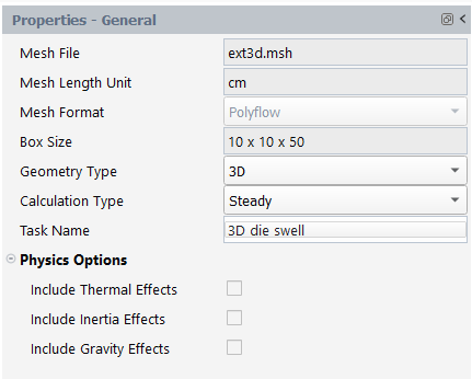
Select General in the Outline View to review general properties of the simulation.
Review the settings in the properties page.
Make sure that Steady is selected for the Calculation Type.
Enter
3D die swellfor the Task Name.
Fluent indicates which material properties are relevant by graying out the irrelevant properties. For this model you will only define the viscosity of the material.
Even though the default material's (fluid) properties are up-to-date, you will change how that material's viscosity is defined.
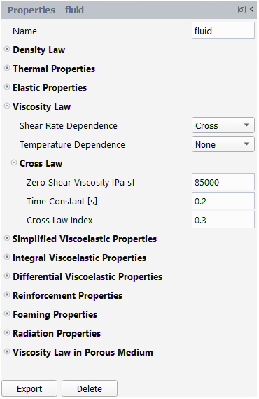
Select fluid under Materials in the Outline View to review material properties of the simulation.
In the Properties - fluid panel, click the icon to the left of the Viscosity Law category to define the viscosity properties of the fluid.
For Shear Rate Dependence, select Cross.
The Cross law exhibits shear-thinning (the decrease in viscosity as the shear rate increases) that is a characteristic of many polymers. The viscosity in this tutorial is given by the Cross law:

(3–1)
where:
 = zero shear-rate viscosity = 85000 poise
  = natural time = 0.2 s
 = Cross law index = 0.3
 = shear rate
For Zero Shear Viscosity
[Pa s], enter85000.For Time Constant
[s], enter0.2.For Cross Law Index, enter
0.3.
In this portion of the tutorial, you will assign your fluid cell zones.
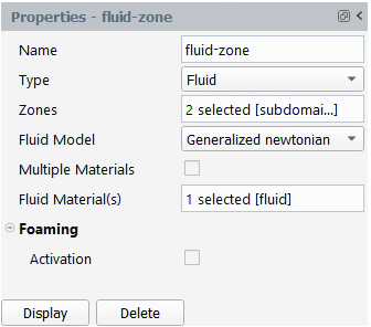
Select fluid-zone under Cell Zones in the Outline View to review cell zone properties of the simulation.
For Zones, select the field to open the ZoneId dialog.
In the ZoneId dialog, select both subdomain1 and subdomain2 and click OK to keep your selections and close the dialog.
In the following steps you will set the conditions at each of the boundaries of the simulation.
Set inlet conditions.
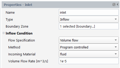
Select inlet under Fluid Boundary Conditions in the Outline View to review inlet boundary conditions for the simulation.
Select boundary1 as the Boundary Zone.
Select Volume Flow as the Flow Specification.
Select fluid as the Incoming material.
Enter
0.00001m^3/s (10 cm^3/s) as the Volume Flow Rate.
Set outlet conditions.
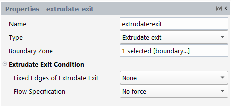
Select extrudate-exit under Fluid Boundary Conditions in the Outline View to review exit boundary conditions for the simulation.
Select boundary6 as the Boundary Zone.
Set symmetry conditions.
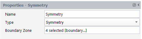
Select Fluid Boundary Conditions in the Outline View, and click the New... button in its properties window, or right-click in the tree and add a new condition to the tree.
Rename the new condition to Symmetry.
Set the Type to Symmetry.
Select boundary3-subdomain1, boundary3-subdomain2, boundary4-subdomain1, and boundary4-subdomain2 as the Boundary Zone.
Set free surface conditions.
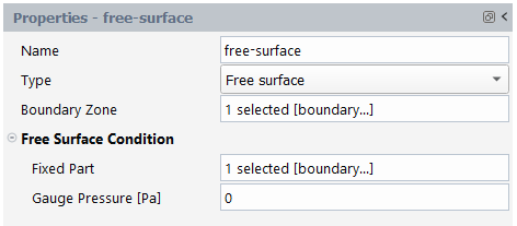
Select free-surface under Fluid Boundary Conditions in the Outline View to review free surface boundary conditions for the simulation.
Select boundary5 as the Boundary Zone.
Select boundary2 as the Fixed Part.
Set wall conditions.
At a solid-liquid interface, the velocity of the liquid is that of the solid surface. Hence the fluid is assumed to stick to the wall. This is known as the no-slip condition because the liquid is assumed to adhere to the wall, and hence, has no velocity relative to the wall.
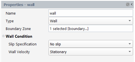
Select wall under Fluid Boundary Conditions in the Outline View to review wall boundary conditions for the simulation.
Select boundary2 as the Boundary Zone.
This model involves a free surface, whose shape is unknown a priori, which will be calculated together with the flow equations. A portion of the mesh is affected by the relocation of this boundary, so a remeshing technique is applied on this part of the mesh. The free surface is entirely contained within subdomain 2, therefore only subdomain 2 is affected by the relocation of the free surface.
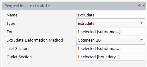
Under Mesh Deformations, select extrudate to edit the default properties of the extrudate exit for your simulation.
Select subdomain2 for Zones.
Select Optimesh-3D for the Extrudate Deformation Method.
Select subdomain2-subdomain1 for the Inlet Section.
Select boundary6 for the Outlet Section.
The purpose of the remeshing technique is to relocate internal nodes according to the displacement of boundary nodes due to the motion of the free surface, since a part of the mesh is deformed. For 3D extrusion problems where large deformations of the extrudate are expected, the optimesh remeshing technique is recommended
The optimesh remeshing technique requires the direction of extrusion
to be parallel to the  ,
,  , or
, or  axis, and all slices into which the remeshing domain is cut must
be perpendicular to the extrusion axis.
axis, and all slices into which the remeshing domain is cut must
be perpendicular to the extrusion axis.
The domain to be remeshed is cut into a series of 2D slices (planes) in a direction perpendicular to the direction of extrusion, and each plane is remeshed independently. For this process, Polyflow requires the selection of the initial plane and the final plane. In this problem, the initial plane is the intersection of subdomain 2 with subdomain 1, and the final plane is the intersection of subdomain 2 with the flow exit (boundary 6).
Open the Solution branch of the Outline View (or use the Ribbon). Here, you can review problem setup and other solution properties. Most items indicate that current default values are appropriate.
Review your problem setup.
Select Run Calculation to see available options.

Click Check to review your simulation settings. Fluent will inform you as to whether or not your setup contains any problems and will provide guidance to solve any issues.
Calculate a solution.
Click Calculate to begin the computing a solution.
Once the calculations are complete, check the solution's listing in the Transcript tab, at the bottom of the Graphics window, to confirm its success. You can confirm that the solution proceeded as expected by looking for the following printed at the bottom of the listing file:
The computation succeeded.
Save the work.
Your work can be preserved using a "session" file - a Materials Processing workspace-specific case file (
*.mprcas) that contains your settings and your results.File → → , entering
extrusion-3Das the name of the session.
Review results using the various tools in the Results section of the Outline View or the Ribbon where you can setup contours, vectors, and so on.
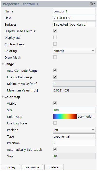
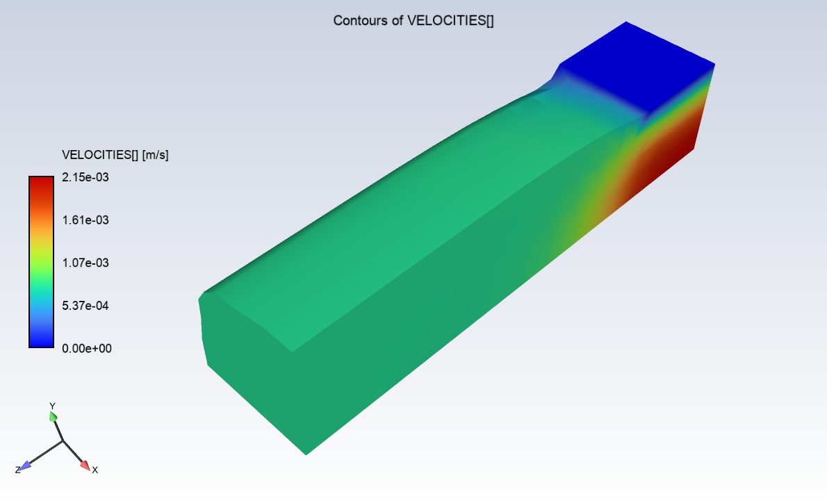
Display the velocity distribution on the boundaries.
Results → Graphics
→ Contour → New Keep the default Name (
contour-1).For the Field, select VELOCITIES[].
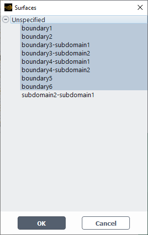
For the Surfaces, select the field to open the Surfaces dialog where you can select the relevant boundaries. Once your selections are complete, click OK to close the dialog.
Keep the remaining defaults and click Display to see the velocity magnitude contour plot in the Graphics window.
Use the toolbars in the Graphics window to adjust the display so that it is in an isometric orientation, and fits the window.
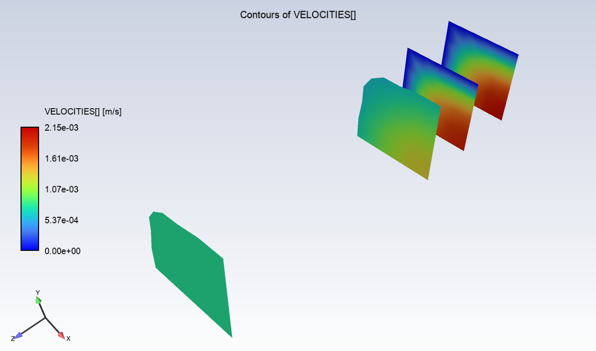
Display contours of velocity in cross-sectional planes, at Z = 0, 0.08, 0.15, and 0.45 m.
Create a cross-section planes at Z = 0 m.
Results
→ Surfaces
→ Plane →
New 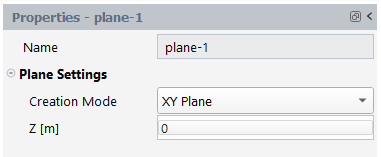
In the Properties - plane-1 panel, under Plane Settings, select XY Plane for the Creation Mode, enter
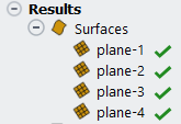
0for Z, and click Display.Create additional cross-section planes for Z = 0.08, 0.15, and 0.45 m.
Once complete, you should have four separate plane surfaces available.
You could also have used the Create Multiple Plane dialog to easily create multiple surfaces.
Display contours of velocity in the cross-sectional planes.
Results → Graphics
→ Contour
→ New 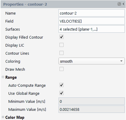
In the properties of contour-2, select VELOCITIES[] for the Field, and for the Surfaces, select the four plane surfaces you just created, keep the remaining defaults, and click Display..
This tutorial introduced the concept of a 3D extrusion problem using the Fluent Materials Processing workspace. You solved the problem using a specific 3D geometry for the die and made suitable assumptions about the physics of the problem. You analyzed the factors affecting the extrudate shape. In addition you learned how to use the optimesh remeshing method, which is recommended for 3D extrusion problems.
This tutorial is divided into the following sections:
This tutorial demonstrates the simulation of a multiple material coextrusion process using the Fluent Materials Processing workspace. A coextrusion process allows for two or more different polymer materials to be combined into a single product. Depending on the materials used, the process allows for the creation of products with unique properties, such as increased strength, resistance to corrosion, or insulation. The versatility of coextruded plastic profiles and tubing makes coextrusion an ideal manufacturing process for a wide range of products.
In this tutorial you will learn how to use the Fluent Materials Processing workspace to set up a coextrusion simulation using multiple materials, calculate the solution, and analyze the results.
This tutorial considers the flow of two different isothermal polymer materials through a three-dimensional die. The problem consists of two inlets, one for each material, which are coextruded through the die to produce a multi-layered tubing structure at the exit.
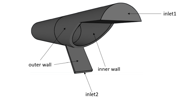
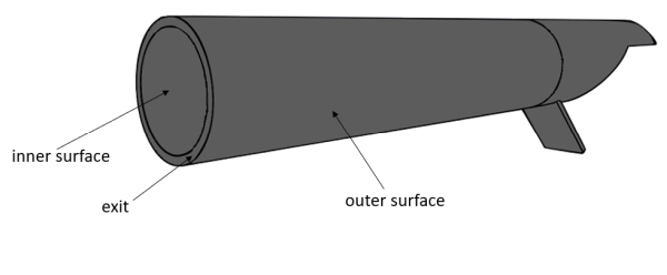
The domain for the problem is divided into two parts, the first part is the die where the two fluid materials are confined between the inner wall and outer wall, as can be seen in Figure 3.7: Problem Description Inlet. The second part corresponds to the multi-material extrudate tubing which is in contact with the air and can deform freely along the inner and outer surfaces, as can be seen in Figure 3.8: Problem Description Exit.
The first inlet (inlet1) is positioned at the top of the die where the first material, high density polyethylene, enters into the domain at a flow rate of Q = 175 * 10 -6 m 3 / s. The second inlet (inlet 2) is positioned at the bottom of the die where the second material, linear low density polyethylene, enters into the domain at a flow rate of Q = 25 * 10 -6 m 3 / s.
At the end of the computational domain, it is assumed that the motion of the multi-material extruded tubing is fully developed and that it will not deform any further. It is assumed that the extrusion domain is long enough to account for the entire deformation of the extrudate.
The following sections describe the setup and solution steps for this tutorial:
To prepare for running this tutorial:
Prepare a working folder for your simulation.
Download the
coextrusion.zipfile here .Unzip the
coextrusion.zipfile you have downloaded to your working folder.The mesh file
coextruded_tubing.mshcan be found in the unzipped folder.
Use the Fluent Launcher to start Ansys Fluent.
Select Materials Processing in the list of Fluent workspaces.
Click Start.
Clicking Start in the Fluent Launcher opens the Fluent Materials Processing workspace.
Open the geometry by reading in a Polyflow mesh file.
In the Setup properties, under Read, click the Mesh... button.
You can also use the File menu, and choose Read > Polyflow Mesh....
Locate and select the mesh file from your working folder (
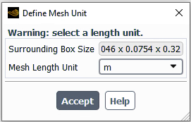
coextruded_tubing.msh)Set the Mesh Length Unit to m, and close the dialog box.
Set up an extrusion simulation (using the Simulation category of the Setup Ribbon).
Setup
→ Simulation → Use
Template...
This will display the Simulation Template dialog.
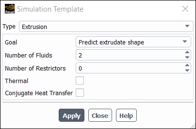
Set the Type to Extrusion.
Set the Goal to be Predict extrudate shape.
Enter
2for the Number of fluids.Click Apply.
This will instruct the workspace to set up the appropriate objects and settings based on your selections.
Note: Notice the Outline View's use of status icons. A green check mark indicates the properties of that object are satisfactory. A red 'x' indicates that attention is required for that object.
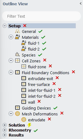
You can progress down the Outline View (or across the Ribbon) to complete your simulation settings using each object's property pages.
Display and review the general settings for the problem setup.
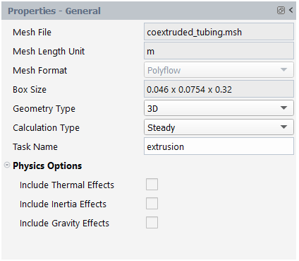
Select General in the Outline View to review general properties of the simulation.
Review the settings in the properties page.
Make sure that Steady is selected for the Calculation Type.
For this tutorial, you will replace the two fluids that were created for you with two materials imported from an installed material library.
Import a new material from the materials library.
Click the Import from library button in the Materials property page. Alternatively, you can right-click on the Materials node, and select Import from library from the context menu.
 Materials
  Import
from library
Import
from library This displays the Library of Materials dialog box.
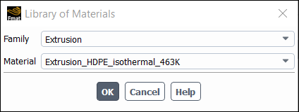
Select Extrusion for the Family.
Select Extrusion_HDPE_isothermal_463K for the Material.
Click OK to close the dialog.
The new material will be added to the list of materials in the Outline View.
Import another material from the library by repeating the same procedure.
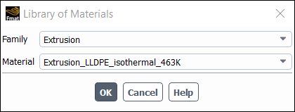
Select Extrusion for the Family
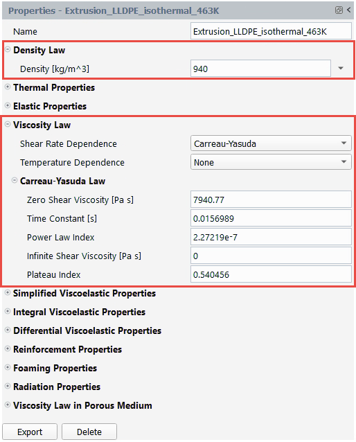
Select Extrusion_LLDPE_isothermal_463K for the Material.
Click OK to close the dialog.
The new material will be added to the list of materials in the Outline View.
Remove the original fluid materials (fluid-1 and fluid-2).
Select fluid-1 in the Outline View, right-click and select Delete from the context menu.
Setup →
Materials →
fluid-1
Delete
You will be prompted to make sure you want to remove the material. Click Yes to remove the material.
Perform the same operation for fluid-2 to remove it from your setup.
Review material properties.
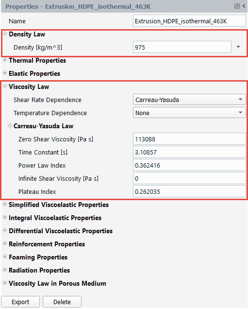
Select Extrusion_HDPE_isothermal_463K under Materials in the Outline View to review material properties of the simulation.
Review the density and the viscosity settings for the first material.
Review the density and the viscosity settings for the Extrusion_LLDPE_isothermal_463K material.
In this portion of the tutorial, you will assign your fluid cell zones.
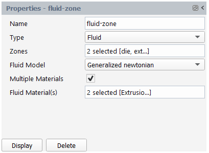
Select fluid-zone under Cell Zones in the Outline View to review cell zone properties of the simulation.
For Zones, select the field to open a selection dialog.
In the selection dialog, select both available zones: die and extrudate and click OK to keep your selections and close the dialog.
For Fluid Material(s), select the field to open a selection dialog.
In the selection dialog, select the two materials previously created: Extrusion_HDPE_isothermal_463K and Extrusion_LLDPE_isothermal_463K and click OK to keep your selections and close the dialog.
In the following steps you will set the conditions at each of the boundaries of the simulation.
Set outlet conditions.
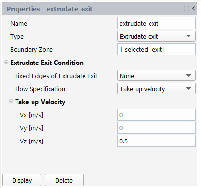
Select extrudate-exit under Fluid Boundary Conditions in the Outline View to review the exit boundary conditions for the simulation.
Select exit as the Boundary Zone.
Select Take-up Velocity as the Flow Specification.
Enter
0m/s for Vx.Enter
0m/s for Vy.Enter
0.5m/s for Vz.
Set free surface conditions.
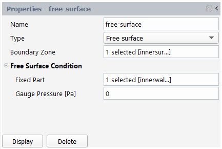
Select free-surface under Fluid Boundary Conditions in the Outline View to review free surface boundary conditions for the simulation.
Select innersurface as the Boundary Zone.
Select innerwall as the Fixed Part.
Define a new free surface boundary.
Click the New... button in the Fluid Boundary Conditions property page. Alternatively, you can right-click on the Fluid Boundary Conditions node, and select New... from the context menu.
Fluid Boundary Conditions
New...
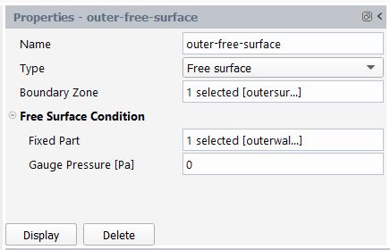
Enter outer-free-surface for the Name.
Select Free surface for the Type.
Select outersurface for the Boundary Zone.
Select outerwall for the Fixed Part.
Set inlet conditions for the Extrusion_HDPE_isothermal_463K material.
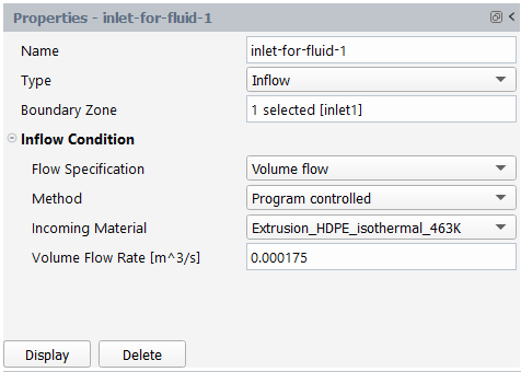
Select inlet-for-fluid-1 under Fluid Boundary Conditions in the Outline View to review inlet boundary conditions for the simulation.
Select inlet1 for the Boundary Zone.
Select Volume Flow for the Flow Specification.
For the Incoming Material, select Extrusion_HDPE_isothermal_463K.
Enter
175e-6m^3/s for the Volume Flow Rate.
Set inlet conditions for the Extrusion_LLDPE_isothermal_463K material.
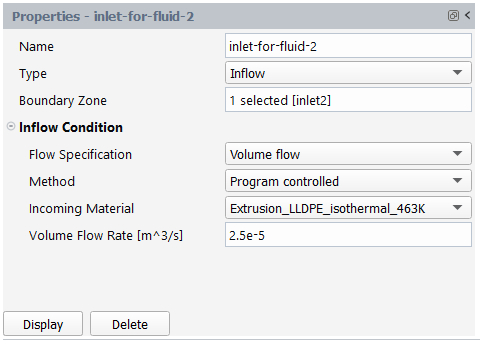
Select inlet-for-fluid-2 under Fluid Boundary Conditions in the Outline View to review inlet boundary conditions for the simulation.
Select inlet2 for the Boundary Zone.
Select Volume Flow for the Flow Specification.
For the Incoming Material, select Extrusion_LLDPE_isothermal_463K.
Enter
25e-6m^3/s for the Volume Flow Rate.
Set wall surface conditions.
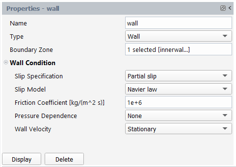
Select wall under Fluid Boundary Conditions in the Outline View to review free surface boundary conditions for the simulation.
Select innerwall as the Boundary Zone.
Select Partial slip for the Slip Specification.
Retain the selection of Navier law for the Slip Model.
Enter
1e6kg/(m^2 s) for the Friction Coefficient.
Define a new wall boundary.
Click the New... button in the Fluid Boundary Conditions property page. Alternatively, you can right-click on the Fluid Boundary Conditions node, and select New... from the context menu.
Fluid Boundary Conditions
New...
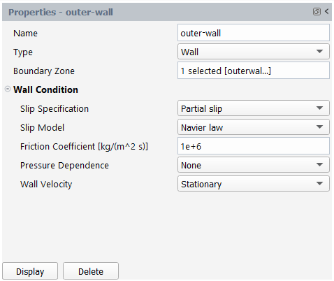
Enter outer-wall for the Name.
Select Wall for the Type.
Select outerwall for the Boundary Zone.
Select Partial slip for the Slip Specification.
Retain the selection of Navier law for the Slip Model.
Enter
1e6kg/(m^2 s) for the Friction Coefficient.
This model involves two free surfaces, whose shape is unknown a priori, which will be calculated together with the flow equations. A portion of the mesh is affected by the relocation of these boundaries, so a mesh deformation technique is applied on this part of the mesh. The extrudate is entirely contained between the inner and outer surfaces, therefore this will be the only zone affected by the mesh deformation algorithm.
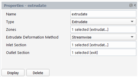
Under Mesh Deformations, select extrudate to edit the default properties of the extrudate exit for your simulation.
Select extrudate for Zones.
Select Streamwise for the Extrudate Deformation Method.
Select extrudate-die for the Inlet Section.
Select exit for the Outlet Section.
Open the Solution branch of the Outline View (or use the Ribbon). Here, you can review problem setup and specify other solution properties.
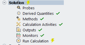
Define the Calculation Activities.
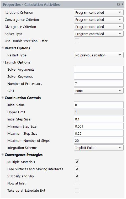
The number of processors is set to 4 by default, which is sufficient for most cases. However, for this problem we will increase the number of processors to 7 which will moderately increase the marginal speedup. Note that the value specified for the processor count does not need to be a power of 2.
Enter 7 for the Number of Processors.
The primary source of non-linearity in a coextrusion flow originates from the transport of immiscible materials and their respective properties. At each location in the calculation domain, equations must be inspected for the appropriate properties assignment. For facilitating the calculation, convergence strategies are available. Next to convergence strategy for multiple materials, which is often recommended for coextrusion flow calculations, we also enable convergence strategies for free surfaces and moving interfaces as well as for viscosity and slip.
Enable the Multiple Materials option.
Enable the Free Surfaces and Moving interfaces option.
Enable the Viscosity and Slip option.
Review your problem setup.
Select Run Calculation to see available options.
Click Check to review your simulation settings. The Fluent Materials Processing workspace will inform you as to whether or not your setup contains any problems and will provide guidance to solve any issues.
Calculate the solution.
Click Calculate to begin the computation of the solution.
Depending on your machine, the calculation should take approximately 20 to 25 minutes to complete.
Once the calculations are complete, check the solution's listing in the Transcript tab to confirm its success. You can confirm that the solution proceeded as expected by looking for the following printed at the bottom of the listing file:
The computation succeeded.
Save the work.
Your work can be preserved using a "session" file - a Materials Processing workspace-specific case file (
*.mprcas) that contains your settings and your results.File → → , entering
coextruded-tubingas the name of the session.
Review results using the various tools in the Results section of the Outline View or the Ribbon where you can setup contours, vectors, and so on.
Display the fluid fraction distribution on the boundaries.
Results → Graphics
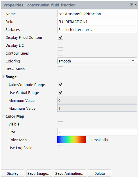
→ Contour → New The fluid fraction distibution (FLUIDFRACTION1) represents the proportion or fraction of fluid material within the multi-layered tubing.
For the Name, enter
coextrusion-fluid-fraction.For the Field, select FLUIDFRACTION1.
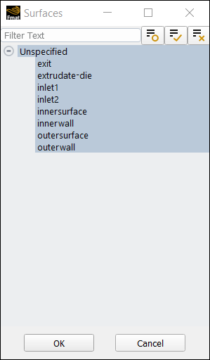
For the Surfaces, select the field to open the Surfaces dialog where you can select the relevant boundaries. Once your selections are complete, click OK to close the dialog.
Keep the remaining defaults and click Display to see the fluid fraction contour plot in the graphics window.
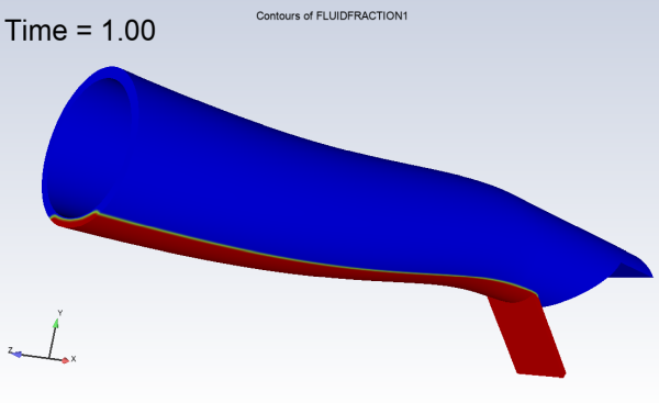
In Figure 3.11: Contours of FLUIDFRACTION1 we can see the high density polyethylene in blue, and the linear low density polyethylene in red. The interface between these two polymers is shown in green. A more refined mesh in the zone where the fluid fraction varies will improve the interface location.
This tutorial is divided into the following sections:
This tutorial illustrates the simulation of a 3D blow molding process using the Fluent Materials Processing workspace (Fluent Materials Processing Workspace). The workspace will allow you to set up and solve a polymer blow molding problem so you can easily obtain an accurate prediction of the shaped object for a given mold geometry under prescribed operating conditions.
In this tutorial you will learn how to use the Fluent Materials Processing workspace to:
Easily set up your blow molding / thermoforming simulation
Calculate a solution
Analyze the results, such as generating thickness-based contour plots and running transient animations.
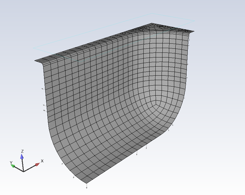
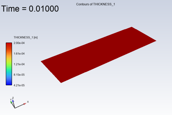
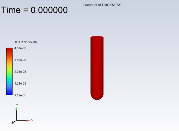
This tutorial simulates a typical thermoforming situation for a blister. Figure 3.12: Thermoforming of a Blister, Sheet (blue) and Mold (red) shows a view of the process in the initial configuration.
To reduce the computational run time, and utilizing the symmetric nature of the blister, only one quarter of the blister/mold is modeled, Figure 3.12: Thermoforming of a Blister, Sheet (blue) and Mold (red). From a geometric point of view, the initial (1/4) film has the following dimensions:
Length = 0.015 m
Width = 0.05 m
Initial thickness = 0.0005 m
This tutorial demonstrates the modeling of a polymer sheet made up of several layers, as it is often the case for packaging food or medication, where one layer provides mechanical resistance and another layer provides a humidity barrier.
The thickness of the layer, when compared to the length/width of the blister, is rather small. This allows for the use of the membrane (shell) element, which is suited for the analysis of 3D blow molding and thermoforming simulations. The use of the membrane element is presently restricted to time-dependent flows and is combined with Lagrangian representation (each mesh node is a material point). Node displacement results from the time integration of nodal velocity.
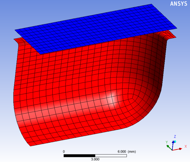
The finite element mesh and the boundary conditions are displayed in Figure 3.13: Finite Element Mesh, Subdomains and Boundary Sets. A 3D surface mesh has been generated for both the mold and the film. The most important aspect is the proper description of the inner mold surfaces that will shape the blister.
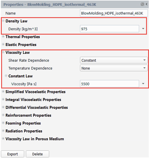
The film has the following material properties:
First layer: Viscosity = 5500 Pa -s
Second layer: Viscosity = 4000 Pa -s
First layer: Density = 975 kg/m3
Second layer: Density = 1100 kg/m3
First layer: Initial thickness = 0.0002 m
Second layer: Initial thickness = 0.0003 m
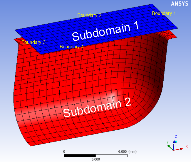
As seen in Figure 3.13: Finite Element Mesh, Subdomains and Boundary Sets, the topology involves two subdomains:
Subdomain 1 = film
Subdomain 2 = mold
and four boundary sets:
Boundary 1: will be fixed (clamped boundary)
Boundary 2: will be fixed (clamped boundary)
Boundary 3: symmetry boundary condition with respect to the x-axis
Boundary 4: symmetry boundary condition with respect to the y-axis
The inflation pressure will be defined on the subdomain representing the film (Subdomain 1).
When considering contact with a mold, typically, two cases may be encountered:
The moving mold comes in contact with the shell and the shell acquires the mold velocity.
The shell is inflated according to a certain rate and eventually comes into contact with the mold, acquiring its shape.
Often, both types of contact are encountered in a given application.
The following sections describe the setup and solution steps for this tutorial:
- 3.3.3.1. Preparation
- 3.3.3.2. Launching Ansys Fluent
- 3.3.3.3. Setup Your Simulation
- 3.3.3.4. General Properties
- 3.3.3.5. Material Properties
- 3.3.3.6. Cell Zone Properties
- 3.3.3.7. Layer Properties
- 3.3.3.8. Fluid Boundary Condition Properties
- 3.3.3.9. Contact Boundary Conditions
- 3.3.3.10. Mesh Deformation Properties
- 3.3.3.11. Adaptive Mesh Settings
- 3.3.3.12. Solution
To prepare for running this tutorial:
Prepare a working folder for your simulation.
Download the
3d_thermo_blister.zipfile here .Unzip the
3d_thermo_blister.zipfile you have downloaded to your working folder.The mesh file
blister.mshcan be found in the unzipped folder.
Use the Fluent Launcher to start Ansys Fluent.
Select Materials Processing in the list of Fluent workspaces.
Click Start.
Clicking Start in the Fluent Launcher opens the Fluent Materials Processing workspace.
The workspace is a version of Ansys Fluent that utilizes the power of the Ansys Polyflow solver to simulate polymer flows such as extrusion, blow molding, pressing, and so forth.
Open a blow molding geometry by reading in a Polyflow mesh file.
In the Setup properties, under Read, click the Mesh... button.
You can also use the File menu, and choose Read > Polyflow Mesh....
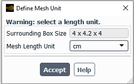
Locate and select the mesh file from your working folder (
blister.msh)In this case, the mesh file does not contain any unit information, so you are prompted to provide the units through the dialog. Set the Mesh Length Unit to mm, and close the dialog box.
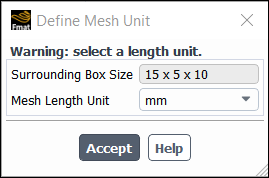
Note: The Fluent Materials Processing workspace always performs the setup and the calculations in MKS. If the mesh is provided in other units, then the coordinates are converted to meters prior to the calculation.
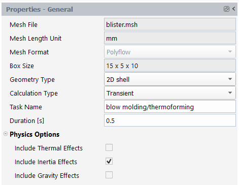
Set up a blow molding simulation (using the Simulation category of the Setup Ribbon).
Setup
→ Simulation → Use
Template...
This will display the Simulation Template dialog.
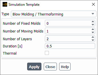
Set the Type to Blow Molding / Thermoforming.
Keep the Number of Fixed Molds as
0.Set the Number of Moving Molds to
1.Set the Number of Layers to
2.Set the Duration to
0.5seconds.Click Apply.
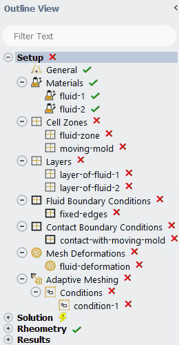
This will instruct the workspace to set up the appropriate objects and settings based on your selections.
Note: Notice the Outline View's use of status icons. A green check mark indicates the properties of that object are satisfactory. A red 'x' indicates that attention is required for that object.
You can progress down the Outline View (or across the Ribbon) to complete your simulation settings using each object's property pages.
Click the General node in the Outline View to display general settings for the problem setup. For this tutorial, you can keep the default settings.
For this tutorial, you will replace the two fluids that were created for you with two special materials imported from an installed material library.
Import a new material from the materials library.
Click the Import from library button in the Materials property page. Alternatively, you can right-click on the Materials node, and select Import from library from the context menu.
Materials
Import from library This displays the Library of Materials dialog box.
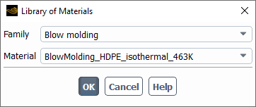
Select Blow molding for the Family
Select BlowMolding_HDPE_isothermal_463K for the Material.
Click OK to close the dialog.
The new material will be added to the list of materials in the Outline View.
Import another material from the library by repeating the same procedure.
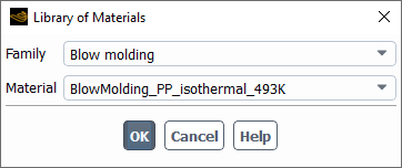
Select Blow molding for the Family
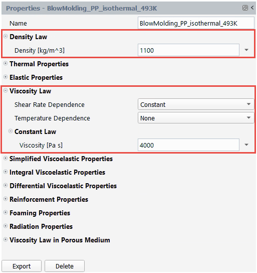
Select BlowMolding_PP_isothermal_493K for the Material.
Click OK to close the dialog.
The new material will be added to the list of materials in the Outline View.
Remove the original fluid materials (fluid-1 and fluid-2).
Select fluid-1 in the Outline View, right-click and select Delete from the context menu.
Setup →
Materials →
fluid-1
Delete
You will be prompted to make sure you want to remove the material. Click Yes to remove the material.
Perform the same operation for fluid-2 to remove it from your setup.
Review material properties.
Select BlowMolding_HDPE_isothermal_463K under Materials in the Outline View to review material properties of the simulation.
When you select an item in the Outline View, you can see and edit its properties and settings in the separate Properties View window. There are numerous material properties available for your materials using the workspace. Material properties are listed by category and you can expand the properties of the categories you are interested in by clicking the icon to the left of the category.
Review the density and the viscosity settings for the first material.
Review the density and the viscosity settings for the second material.
In this portion of the tutorial, you will assign which cell zone is the fluid which is the moving mold, and prescribe the motion of the mold using an expression.
Set the cell zone conditions for the fluid zone.
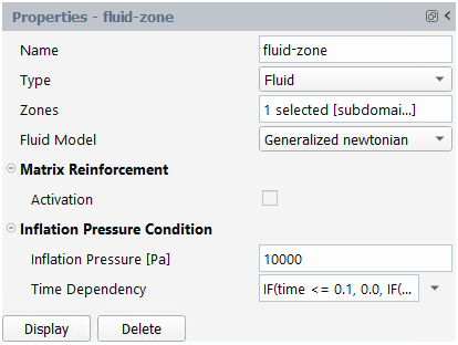
Select fluid-zone under Cell Zones in the Outline View to review cell zone properties of the simulation.
For Zones, select the field to open a selection dialog. In the selection dialog, select subdomain1 and click OK to keep your selections and close the dialog.
Set the Inflation Pressure to
10000Pa.Click Display to visualize arrows on the fluid zone that demonstrate the orientation of the pressure.
Select expression from the Time Dependency drop-down list, then enter
IF(time <= 0.1, 0.0, IF(time >= 0.11, 1.0,
                                    (time-0.1)/(0.11-0.1)))
for the time dependency.
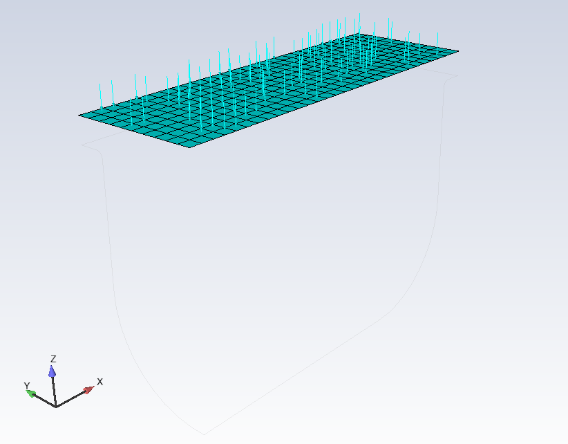
Set the cell zone conditions for the moving mold zone.
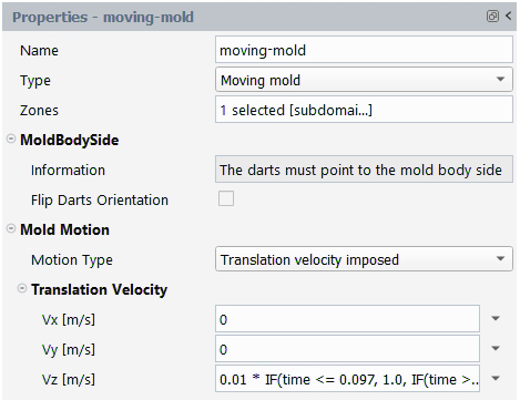
Select moving-mold under Cell Zones in the Outline View to review cell zone properties of the simulation.
For Zones, select the field to open a selection dialog. In the selection dialog, select subdomain2 and click OK to keep your selections and close the dialog.
Check the orientation.
Click Display to visualize arrows on the moving mold zone that demonstrate the orientation, and to confirm that the arrows are pointing to the mold body.
Under Translation Velocity, select expression from the Vz drop-down list and enter
0.01 * IF(time <= 0.097,
                                    1.0, IF(time >= 0.103, 0.0, 17.167 - time *
                                    166.67))
for Vz.
Using the blow molding simulation template, this tutorial defined two layers. In the following steps you will further define the various layers of the simulation, each having its own material properties and initial thickness (which can be defined as a constant, or a linear function of X, Y, Z coordinates. Layers can overlap (partly or entirely), but they are not required to do so. Here, each layer is defined on the same fluid-zone. The solver will model the deformation of the polymer sheet that combines (the resistance of) the two layers. The layers are meant to stick together, so the deformation of each layer is identical, since the area stretch can only be computed once.
Set conditions for the first layer.
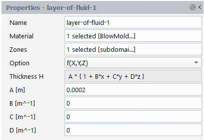
Select layer-of-fluid-1 under Layers in the Outline View to review this layer's settings for the simulation.
Select BlowMolding_HDPE_isothermal_463K as the Material.
Select subdomain1 as the Zones.
Select f(X,Y,Z) under Option.
The layer's thickness H is defined by the polynomial:
A*(1+B*x+C*y+D*z). All that is required for this tutorial is a value for the first coefficient, A, so enter0.0002m.
Set conditions for the second layer.
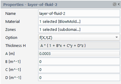
Select layer-of-fluid-2 under Layers in the Outline View to review this layer's settings for the simulation.
Select BlowMolding_PP_isothermal_493K as the Material.
Select subdomain1 as the Zones.
Select f(X,Y,Z) under Option.
Enter
0.0003m for the thickness coefficient A.
In the following steps you will set the conditions at each of the boundaries of the simulation.
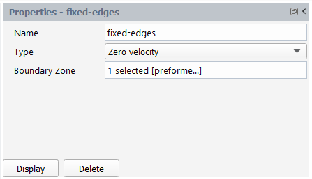
Set conditions for the fixed edges.
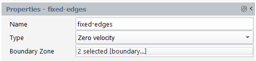
Select fixed-edges under Fluid Boundary Conditions in the Outline View to review this boundary condition for the simulation.
Select boundary1 and boundary2 as the Boundary Zone.
Set two symmetry conditions.
Select Fluid Boundary Conditions in the Outline View, and click the New... button in its properties window, or right-click in the tree and add a new condition to the tree.
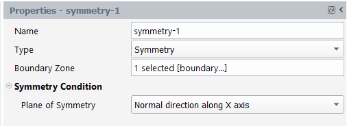
Rename the new condition to symmetry-1.
Set the Type to Symmetry.
Select boundary3 as the Boundary Zone.
Select Normal direction along X axis as the Plane of Symmetry.
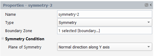
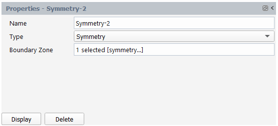
Repeat the process and assign a symmetry boundary called symmetry-2 to boundary4, assigning its plane of symmetry to be Normal direction along Y axis.
Contact between the fluid film and the solid mold can be accounted for using contact conditions.
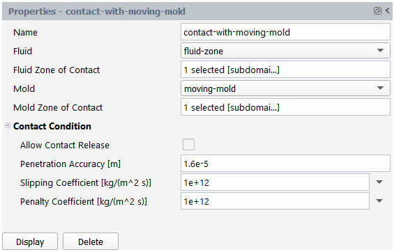
Under Contact Boundary Conditions, select contact-with-moving-mold to edit the default properties of this contact condition for your simulation.
Select subdomain1 for the Fluid Zone of Contact.
Select subdomain2 for the Mold Zone of Contact.
Here, we'll assign the film cell zone to be a deforming fluid.
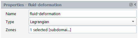
Under Mesh Deformations, select fluid-deformation to edit the default properties of the fluid deformation zone for your simulation.
Select subdomain1 for Zones.
In many practical cases, the use of adaptive meshing based on contact, remeshing, or both may be useful to selectively and automatically refine the mesh during the solution. The blow molding simulation template automatically includes adaptive mesh refinement, however, it is not necessary for this tutorial.
Select Adaptive Meshing in the Outline View and disable it in the properties window.
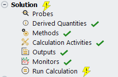
Open the Solution branch of the Outline View (or use the Ribbon). Here, you can review problem setup and other solution properties. Most items indicate that current default values are appropriate.
Review the derived quantities.
Select Derived Quantities to see available options.
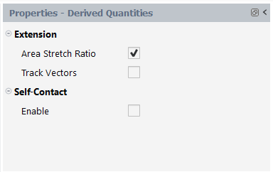
Under Extension, leave the Area Stretch Ratio enabled and retain all other default settings.
Review your problem setup.
Select Run Calculation to see available options.
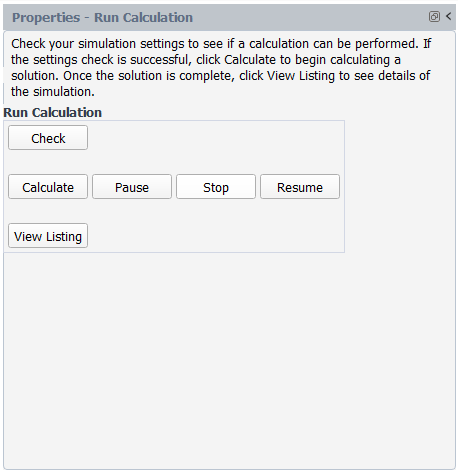
Click Check to review your simulation settings. Fluent will inform you as to whether or not your setup contains any problems and will provide guidance to solve any issues.
Calculate a solution.
Click Calculate to start the calculation.
Once the calculations are complete, check the solution's listing in the Transcript tab to confirm it's success. You can confirm that the solution proceeded as expected by looking for the following printed at the bottom of the listing file:
The computation succeeded.
Save the work.
Your work can be preserved using a "session" file - a Materials Processing workspace-specific case file (
*.mprcas) that contains your settings and your results.File → → , entering
blisteras the name of the session
Review results using the various tools in the Results section of the Outline View or the Ribbon where you can setup contours, vectors, and so on.
Improve the view of the geometry using mirror planes.
Open the Results tab of the Ribbon and, under Graphics, select Mirror Planes... to open the Mirror Planes dialog.
Results → Graphics
→ Mirror Planes...
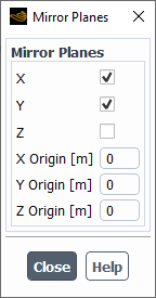
In the Mirror Planes dialog, select X and Y and click Close to close the dialog.
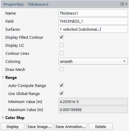
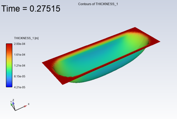
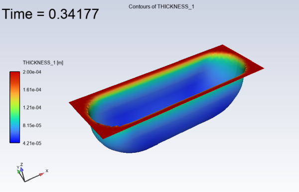
Display contours of thickness (THICKNESS_1) in the fluid region (subdomain1).
Results → Graphics
→ Contour → New Specify a new Name (
Thickness1).For the Field, select THICKNESS_1.
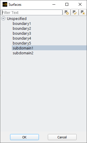
For the Surfaces, select the field to open the Surfaces dialog where you can select the relevant boundaries. Select subdomain1 from the list, and click OK to close the dialog.
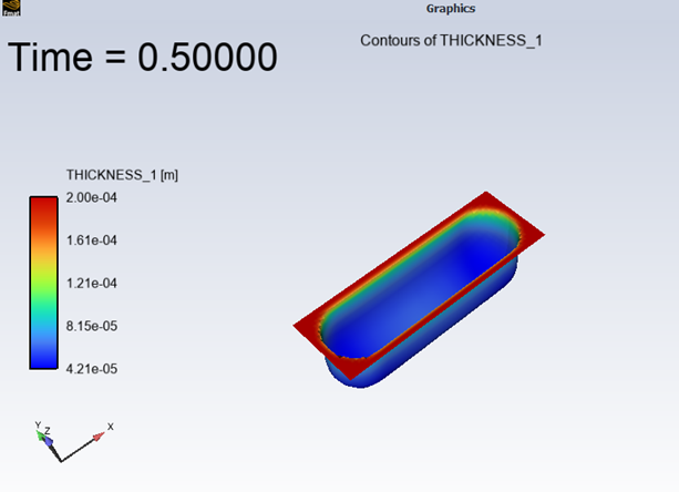
For the contour properties, keep the remaining defaults and click Display to see the thickness contour plot in the Graphics window.
Use the toolbars in the Graphics window to adjust the display so that it is in an isometric orientation, and fits the window.
Review an animation of the contour.
Results → Timestep
To reset the timesteps, change the Current animation time step value to
1. Alternatively, you can also move the slider all the way to the left, or click the Jump to Start button ( ).
).To start the animation., click the Play button (
 )
to start the animation.
)
to start the animation.To stop the animation., click the Stop button (
 ).
).
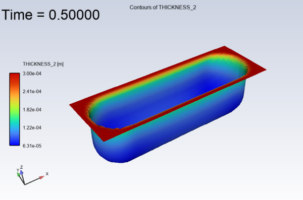
Display contours of thickness (THICKNESS_2) in the fluid region (subdomain1).
Results → Graphics
→ Contour → New Repeat the previous steps to create a new contour over the subdomain1 surface with the Name of
Thickness2with the Field set to THICKNESS_2.Repeat the previous steps to review an animation of the contour.
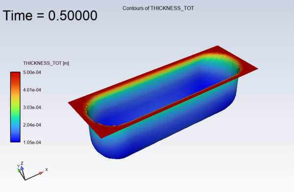
Display contours of thickness (THICKNESS_TOT) in the fluid region (subdomain1).
Results → Graphics
→ Contour → New Repeat the previous steps to create a new contour over the subdomain1 surface with the Name of
Thicknesswith the Field set to THICKNESS_TOT.Repeat the previous steps to review an animation of the contour.
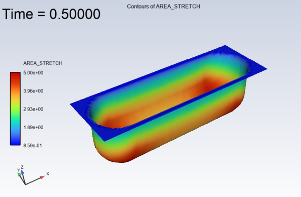
Display contours of area stretch (AREA_STRETCH) in the fluid region (subdomain1).
Results → Graphics
→ Contour → New Repeat the previous steps to create a new contour over the subdomain1 surface with the Name of
AreaStretchwith the Field set to AREA_STRETCH.Repeat the previous steps to review an animation of the contour.
This tutorial introduced the concept of a 3D blow molding problem using the Fluent Materials Processing workspace. You solved the problem using a 3D shell geometry for the mold and the film and made suitable assumptions about the physics of the problem. The mold moved into contact with the film, where a constant pressure was applied to the film. This blew the film into the mold where it assumed the shape of the mold.
This tutorial is divided into the following sections:
This tutorial illustrates the simulation of a 3D injection stretch blow molding (ISBM) process using the Fluent Materials Processing workspace (Fluent Materials Processing Workspace). The workspace will allow you to set up and solve a polymer ISBM problem so you can easily obtain an accurate prediction of the shaped object for a given mold geometry under prescribed operating conditions.
In this tutorial you will learn how to use the Fluent Materials Processing workspace to:
Easily set up your injection stretch blow molding (ISBM) simulation.
Calculate a solution.
Analyze the results, such as generating thickness-based contour plots and running transient animations.
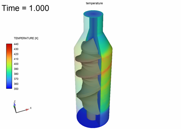
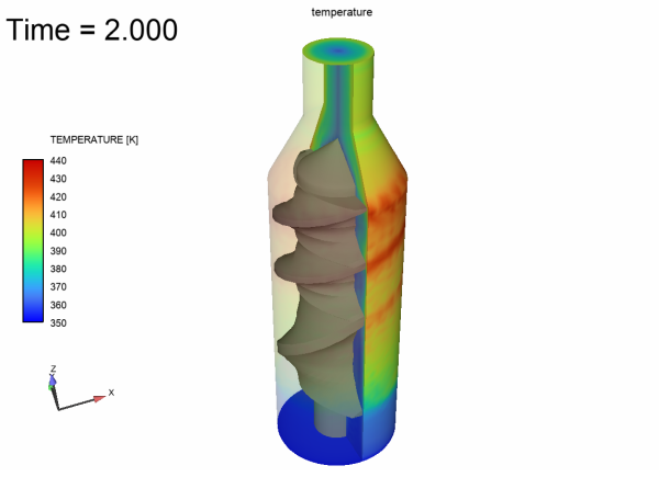
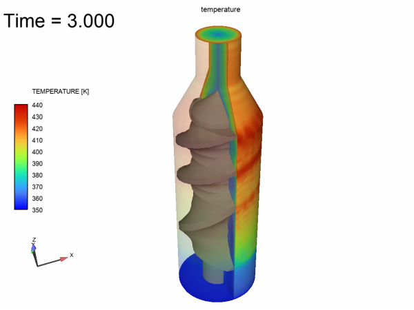
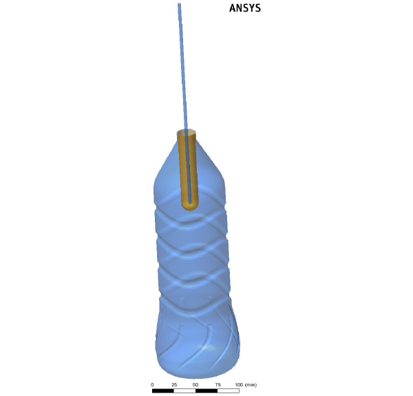
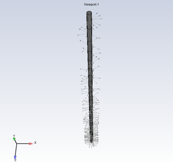
This tutorial covers the injection stretch blow molding (ISBM) process for a 3D bottle. A preform is first set into a mold and stretched by means of a moving rod. Once the rod has reached the desired position (near the bottom of the mold), an internal pressure is applied to the preform to obtain the desired bottle shape. The initial configuration of the model is shown in Figure 3.23: Problem Description and consists of the following three domains:
preform (displayed in orange)
mold (displayed in light blue)
rod (displayed in light blue)
The dimensions of the domains listed above are as follows:
Rod diameter =
0.02mRod height =
0.1mMold diameter =
0.097mMold height =
0.3mPreform initial thickness =
0.005m
The grooves which are visible on the mold suggest that the model does not involve any geometric symmetry.
For this problem, contact release between the preform and the rod is assumed upon application of the shaping pressure. During the tutorial setup, the contact release will be defined using contact boundary conditions and cell zone and fluid boundary conditions will be specified to account for the following:
The velocity-driven motion of the rod during a prescribed time interval (until the rod has reached the specified displacement).
The applied shaping pressure.
Additionally, the following properties will be specified during the tutorial setup:
Downward velocity of the rod =
0.246m/sThis velocity ensures that the rod reaches a position of
0.2m into the mold within0.8s, prior to applying the internal pressure to the preform.Preform material density =
1000kg/m3Applied shaping pressure =
106 PaThe shaping pressure will be defined to apply after
0.86seconds, once the rod reaches the desired position within the preform.Adhesion Force =
10PaThis value will be used to express the contact release of the preform from the rod.
Viscosity =
105 Pa s
The following sections describe the setup and solution steps for this tutorial:
- 3.4.3.1. Preparation
- 3.4.3.2. Launching Ansys Fluent
- 3.4.3.3. Setup Your Simulation
- 3.4.3.4. General Properties
- 3.4.3.5. Material Properties
- 3.4.3.6. Cell Zone Properties
- 3.4.3.7. Layer Properties
- 3.4.3.8. Boundary Condition Properties
- 3.4.3.9. Contact Boundary Conditions
- 3.4.3.10. Mesh Deformation Properties
- 3.4.3.11. Adaptive Mesh Settings
- 3.4.3.12. Solution
To prepare for running this tutorial:
Download the
ISBM.zipfile here .Unzip
ISBM.zipto your working directory.The file,
ISBM.mshcan be found in the folder.
Use the Fluent Launcher to start Ansys Fluent.
Select Materials Processing in the list of Fluent workspaces.
Click Start.
Clicking Start in the Fluent Launcher opens the Fluent Materials Processing workspace.
The workspace is a version of Ansys Fluent that utilizes the power of the Ansys Polyflow solver to simulate polymer flows such as extrusion, blow molding, pressing, and so forth.
Load the provided mesh file.
In the Setup properties, under Read, click the Mesh... button.
You can also use the File menu, and choose Read > Polyflow Mesh....
Locate and select the mesh file from your working folder (
ISBM.msh).Set the Mesh Length Unit to m, and click to close the dialog box.
Set up a blow molding simulation (using the Simulation category of the Setup Ribbon).
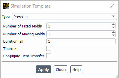
Setup → Simulation
→ Use Template...
This will display the Simulation Template dialog.
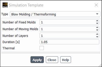
Set the Type to Blow Molding / Thermoforming.
Set the Number of Fixed Molds to 1.
Set the Number of Moving Molds to 1.
Keep the Number of Layers as 1.
Set the Duration to 1.05 seconds.
Click Apply.
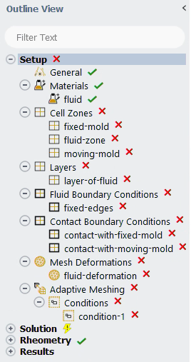
This will instruct the workspace to set up the appropriate objects and settings based on your selections.
Note: Notice the Outline View's use of status icons. A green check mark indicates the properties of that object are satisfactory. A red 'x' indicates that attention is required for that object.
You can progress down the Outline View (or across the Ribbon) to complete your simulation settings using each object's property pages.
Click the General node in the Outline View to display general settings for the problem setup. For this tutorial, you can keep the default settings.
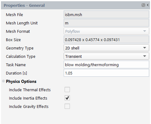
Edit the density and viscosity settings for the fluid material.
Setup →
Materials → fluid
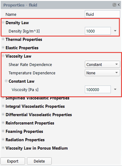
Expand the Density Law and Viscosity Law categories.
In the Density Law category, enter
1000kg/m3 for the Density.In the Viscosity Law category, enter
1e5Pa s for the Viscosity.
In this portion of the tutorial, you will assign your fluid cell zones.
Define the cell zone properties for the fluid-zone.
Setup → Cell
Zones → fluid-zone
For Zones, select the field to open a selection dialog.
In the selection dialog, select preform and click OK to keep the selection and close the dialog.
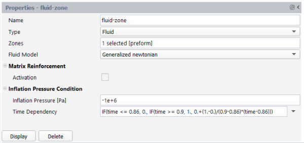
Retain the default selection of Generalized newtonian for Fluid Model .
Enter
-1e6Pa for the Inflation Pressure.Click the arrow next to the Time Dependency entry and select Expression from the drop-down list, then enter the following expression for the time dependency:
IF(time <= 0.86, 0., IF(time >= 0.9, 1.,
                  0.+(1.-0.)/(0.9-0.86)*(time-0.86)))
This expression corresponds to a ramp function which increases from
0to1within the time interval of0.86to0.9.Click Display to visualize arrows on the fluid zone.

The arrows displayed on the fluid-zone show the orientation of the pressure.
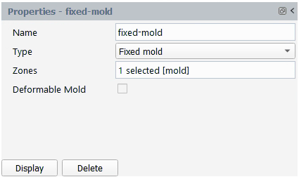
Define the cell zone properties for the fixed-mold.
Setup → Cell
Zones → fixed-mold
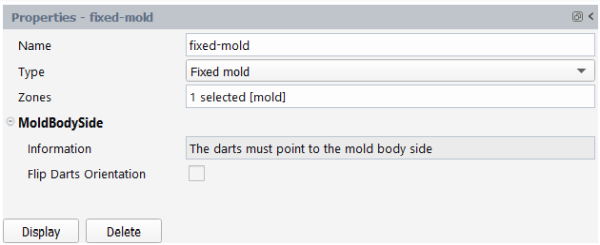
For Zones, select mold.
Click Display to visualize arrows on the fixed mold.
The arrows displayed on the fixed-mold show that the direction is pointing to the mold body side.
Define the cell zone properties for the moving-mold.
Setup → Cell
Zones → moving-mold
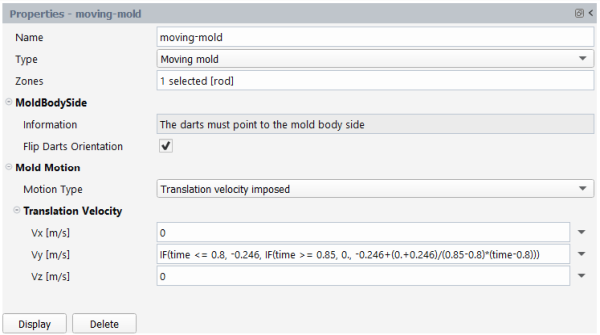
For Zones, select rod.
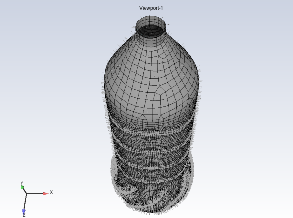
Click Display to visualize the arrows on the rod (moving-mold).
In the Graphics window, rotate the rod to view the arrows from the +Y direction.
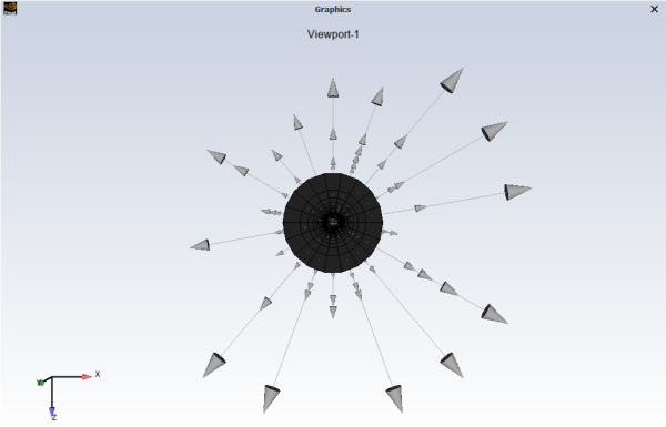
The arrows displayed on the moving-mold point away from the rod, they should point to the rod axis.
Enable the Flip Darts Orientation option to make the arrows point towards the rod.
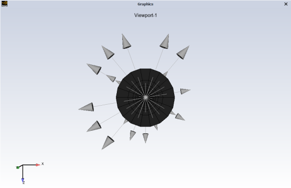
In the above image, the darts may appear to still be facing away from the rod. However, the darts are pointing towards the rod axis, but are overlapping with the rod geometry due to scaling.
Click the arrow next to the Vy entry and select Expression from the drop-down list, then enter the following expression for Vy:
IF(time <= 0.8, -0.246, IF(time >= 0.85, 0.,
                  -0.246+(0.+0.246)/(0.85-0.8)*(time-0.8)))
This expression corresponds to a ramp function which increases from
-0.246to0within the time interval of0.8to0.85.
Define the layer-of-fluid properties.
Setup →
Layers → layer-of-fluid
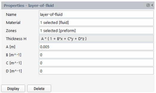
For Zones, select the field to open a selection dialog.
In the selection dialog, select preform and click to keep the selection and close the dialog.
Enter
0.005m as the thickness for A.
Set the conditions for the fixed-edges boundary.
Select fixed-edges under Fluid Boundary Conditions in the Outline View to review this boundary condition for the simulation.
Select preformedge as the Boundary Zone.
Contact between the preform and the solid and moving molds can be accounted for using contact conditions.
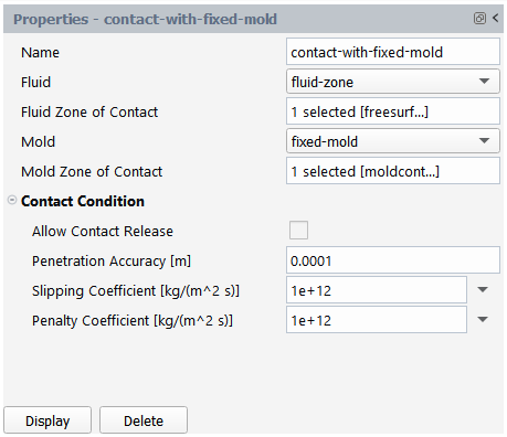
Define the contact between the preform and the fixed mold.
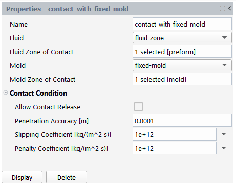
Under Contact Boundary Conditions, select contact-with-fixed-mold to edit the default properties of this contact condition for your simulation.
Select preform for the Fluid Zone of Contact.
Select mold for the Mold Zone of Contact.
Enter
1e-4m for the Penetration Accuracy.
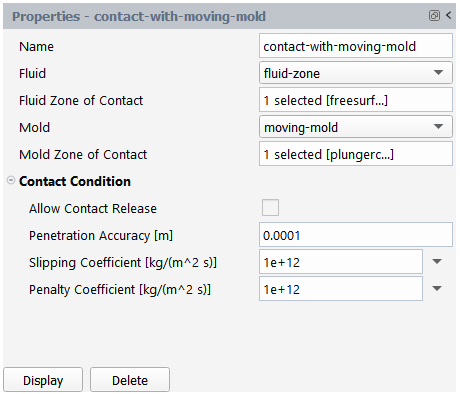
Define the contact between the preform and the moving mold.
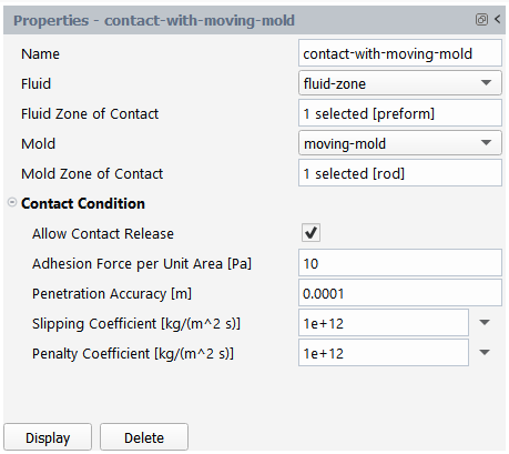
Under Contact Boundary Conditions, select contact-with-moving-mold to edit the default properties of this contact condition for your simulation.
Select preform for the Fluid Zone of Contact.
Select rod for the Mold Zone of Contact.
Enter
1e-4m for the Penetration Accuracy.Enable the Allow Contact Release option.
Enter
10Pa for Adhesion Force per Unit Area.
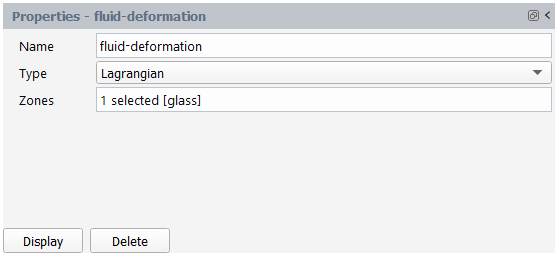
Here, we will assign the preform cell zone to be a deforming fluid.
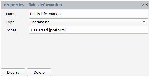
Under Mesh Deformations, select fluid-deformation to edit the default properties of the fluid deformation zone for your simulation.
Retain the selection of Lagrangian as the deformation Type.
Select preform for Zones.
Define the conditions and settings for adaptive meshing that will be used to refine the mesh during the solution.
Define the adaptive meshing condition (condition-1).
Setup → Adaptive
Meshing → Conditions →
condition-1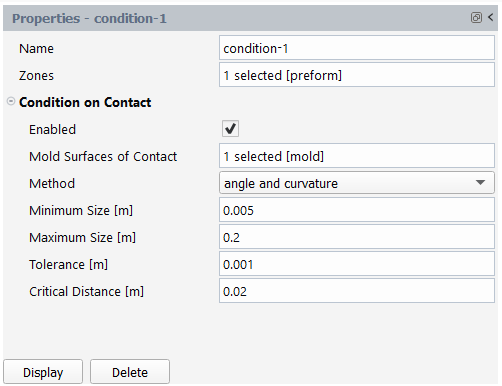
Select preform for Zones.
Select mold for Mold Surfaces of Contact.
Retain the selection of angle and curvature for Method.
Enter
0.005m for Minimum Size.Enter
0.2m for Maximum Size.Enter
0.001m for Tolerance.Enter
0.02m for Critical Distance.
Edit the adaptive meshing properties.
Setup → Adaptive
Meshing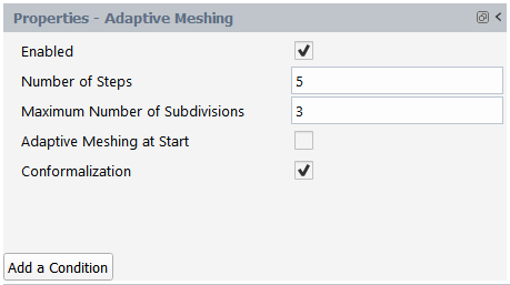
Enter
5for the Number of Steps.
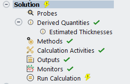
Open the Solution branch of the Outline View (or use the Ribbon). Here, you can review problem setup and other solution properties. Most items indicate that current default values are appropriate.
Edit the Derived Quantities.
Solution → Derived
Quantities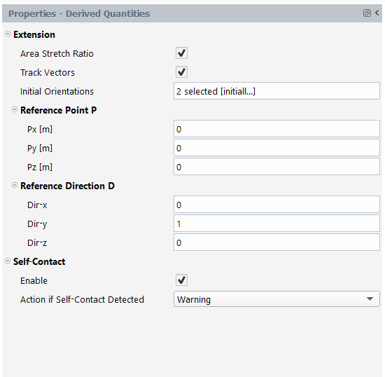
Under Extension, enable the Track Vectors option to expose the additional options.
For Initial Orientation, select initially parallel to D and initially perpendicular to D.
Retain the entry of
0m for reference points Px, Py, and Pz.Enter
0for reference direction Dir-x.Enter
1for reference direction Dir-y.Enter
0for reference direction Dir-z.Enable Self-Contact and retain the selection of Warning for Action if Self-Contact Detected
Edit the Calculation Activities.
Solution → Calculation
Activities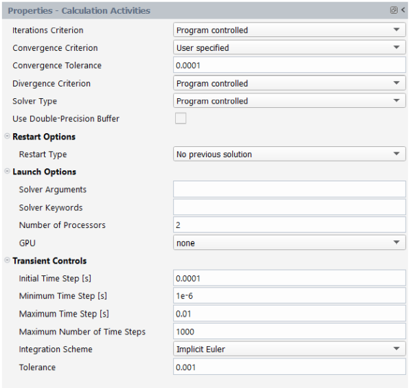
Select Calculation Activities to see available options.
From the Convergence Criterion drop-down list, select User specified.
Enter
0.0001for the Convergence Tolerance.Enter
1e-4seconds for the Initial Time Step.Enter
1e-6seconds for the Minimum Time Step.Enter
1e-2seconds for the Maximum Time Step.Enter
0.001for the Tolerance.
Review your problem setup.
Solution → Run
CalculationClick Check to review your simulation settings. Fluent will inform you as to whether or not your setup contains any problems and will provide guidance to solve any issues.
Calculate a solution.
Click Calculate to start the calculation.
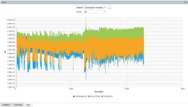
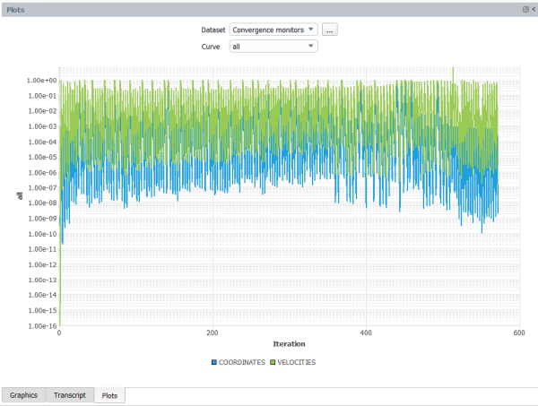
Click the Plots tab to view the plot of the convergence monitors.
Once the calculations are complete, check the solution's listing in the Transcript tab to confirm it's success. You can confirm that the solution proceeded as expected by looking for the following printed at the bottom of the listing file:
The computation succeeded.
Save the work.
Your work can be preserved using a "session" file - a Materials Processing workspace-specific case file (
*.mprcas) that contains your settings and your results.File → → , entering
ISBMas the name of the session
Review results using the various tools in the Results section of the Outline View or the Ribbon where you can setup contours, vectors, and so on.
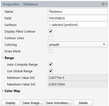
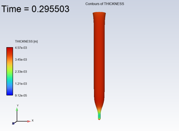
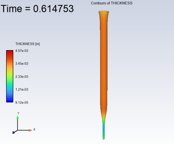
Display contours of thickness (THICKNESS) for the preform surface.
Results → Graphics
→ Contour → New Specify a new Name (
Thickness).For the Field, select THICKNESS.
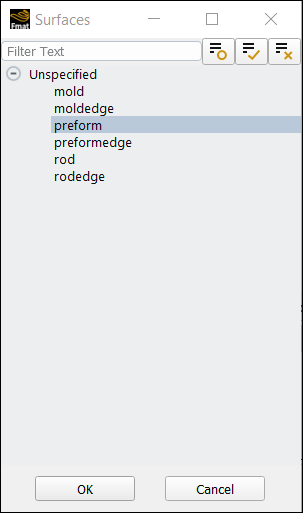
For the Surfaces, select the field to open the Surfaces dialog where you can select the relevant boundaries. Select preform from the list, and click OK to close the dialog.
For the contour properties, keep the remaining defaults and click Display to see the thickness contour plot in the graphics window.
Review an animation of the contour of THICKNESS.
Results → Timestep
To reset the timesteps, change the Current animation time step value to
0. Alternatively, you can also move the slider all the way to the left, or click the Jump to Start button ( ).To start the animation, click the Play button (
).To stop the animation, click the Stop button (
).
Display contours of area stretch (AREA_STRETCH) for the preform surface.
Results → Graphics
→ Contour → New...
Repeat the previous steps to create a new contour over the preform surface with the Name of
AreaStretchwith the Field set to AREA_STRETCH.Repeat the previous steps to review an animation of the contour.
Display contours of self-contact (SELF_CONTACT) for the preform surface.
Results → Graphics
→ Contour → New...
Repeat the previous steps to create a new contour over the preform surface with the Name of
Self-contactwith the Field set to SELF_CONTACT.Repeat the previous steps to review an animation of the contour.
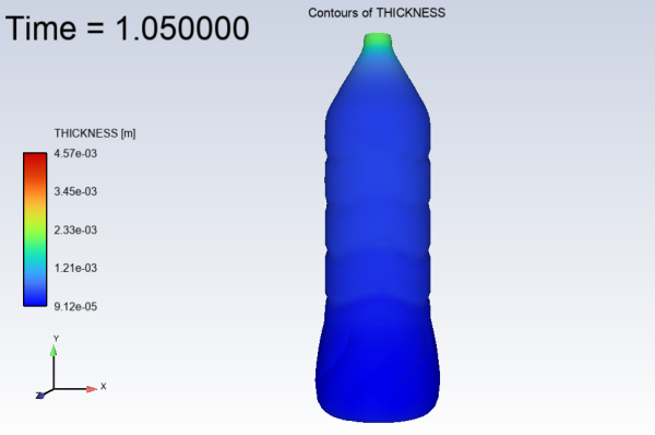
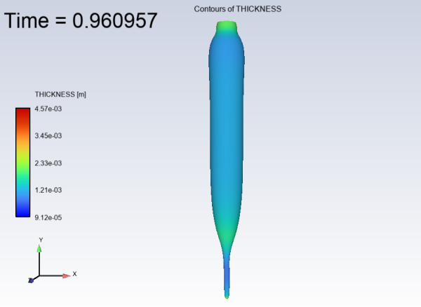
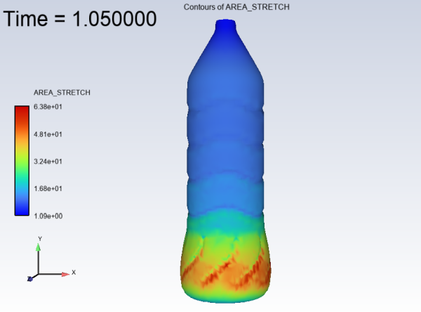
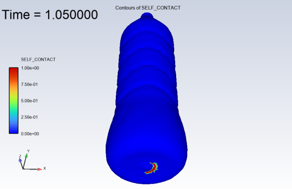
This tutorial introduced the concept of a 3D injection stretch blow molding problem using the Fluent Materials Processing workspace. You solved the problem using a 3D geometry for the mold, the preform, and the moving rod and made suitable assumptions about the physics of the problem. The preform was lowered into a 3D mold using a moving rod, then an internal pressure was applied to obtain the desired bottle shape.
This tutorial is divided into the following sections:
This tutorial illustrates the simulation of a glass pressing process using the Fluent Materials Processing workspace (Fluent Materials Processing Workspace). The workspace will allow you to set up and solve a glass pressing problem so you can easily obtain an accurate prediction of the shaped glass object for a given mold geometry under prescribed operating conditions.
In this tutorial you will learn how to use the Fluent Materials Processing workspace to:
Easily set up your pressing simulation.
Calculate a solution.
Analyze the results, such as generating contour plots and running transient animations.
In this tutorial, we simulate a simple isothermal glass pressing process. In particular, deformations undergone by the fluid as well as contact evolution are investigated. Due to the large deformations involved in the pressing process, adaptive remeshing will also be applied for the fluid zone.
The number of steps between each mesh adaption will be set to 5.
This value is chosen to allow the time step adaption algorithm to reduce or increase the time
step according to the accuracy of the transient scheme.
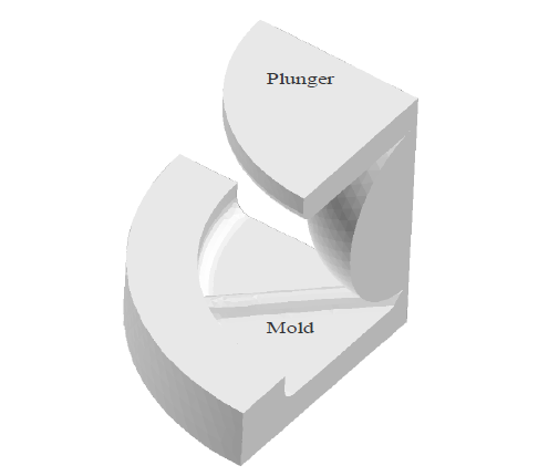
Figure 3.33: Problem Description shows a sketch of the geometry in the initial configuration, before pressing the fluid. A gob of material is placed onto a mold and at a specified time, the plunger moves downwards and presses the fluid volume. Due to the symmetry of the molds and the fluid gob, only a quarter of the geometry is modelled.
From a geometrical point of view, the mesh within three volumes is made of tetrahedra. In
the initial configuration, the plunger is at rest and has a mass of
100 kg. At the start of the process, a constant downward force of
10 N is applied. As the process progresses, the downward velocity
of the plunger varies to maintain the applied force against the viscous forces of the fluid,
which resist deformation. Additionally, the plunger has a maximum displacement of
0.027 m.
The fluid has a constant viscosity of 500 Pa s and density of
2500 kg/m3. It is assumed
that the fluid material sticks on walls while establishing contact with the plunger and the
fixed mold. The contact condition between the fluid and both the plunger and fixed mold will
be defined with a penetration accuracy of 1e-4 m.
The following sections describe the setup and solution steps for this tutorial:
- 3.5.3.1. Preparation
- 3.5.3.2. Launching Ansys Fluent
- 3.5.3.3. Setup Your Simulation
- 3.5.3.4. General Properties
- 3.5.3.5. Material Properties
- 3.5.3.6. Cell Zone Properties
- 3.5.3.7. Boundary Condition Properties
- 3.5.3.8. Contact Boundary Conditions
- 3.5.3.9. Mesh Deformation Properties
- 3.5.3.10. Adaptive Mesh Settings
- 3.5.3.11. Solution
To prepare for running this tutorial:
Download the
glass_pressing.zipfile here .Unzip
glass_pressing.zipto your working directory.The file,
glass_pressing.mshcan be found in the folder.
Use the Fluent Launcher to start Ansys Fluent.
Select Materials Processing in the list of Fluent workspaces.
Click Start.
Clicking Start in the Fluent Launcher opens the Fluent Materials Processing workspace.
The workspace is a version of Ansys Fluent that utilizes the power of the Ansys Polyflow solver to simulate flows of complex rheology fluids and covers processes such as extrusion, blow molding, pressing, and so forth.
Load the provided mesh file.
In the Setup properties, under Read, click the Mesh... button.
You can also use the File menu, and choose Read > Polyflow Mesh....
Locate and select the mesh file from your working folder (
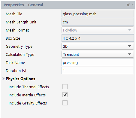
glass_pressing.msh).Set the Mesh Length Unit to cm, and click to close the dialog box.
Set up a pressing simulation (using the Simulation category of the Setup Ribbon).
Setup → Simulation
→ Use Template...
This will display the Simulation Template dialog.
Set the Type to Pressing.
Set the Number of Fixed Molds to 1.
Set the Number of Moving Molds to 1.
Click Apply.
This will instruct the workspace to set up the appropriate objects and settings based on your selections.
Note: Notice the Outline View's use of status icons. A green check mark indicates the properties of that object are satisfactory. A red 'x' indicates that attention is required for that object.
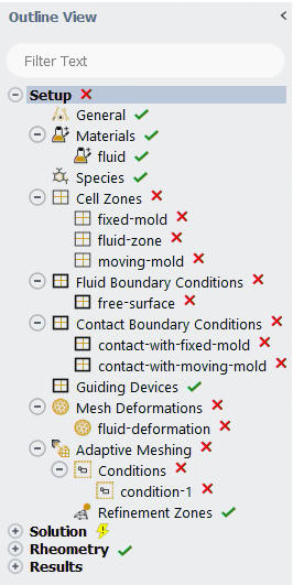
You can progress down the Outline View (or across the Ribbon) to complete your simulation settings using each object's property pages.
Click the General node in the Outline View to display general settings for the problem setup. For this tutorial, you can keep the default settings.
Edit the density and viscosity settings for the fluid material.
Setup →
Materials → fluid
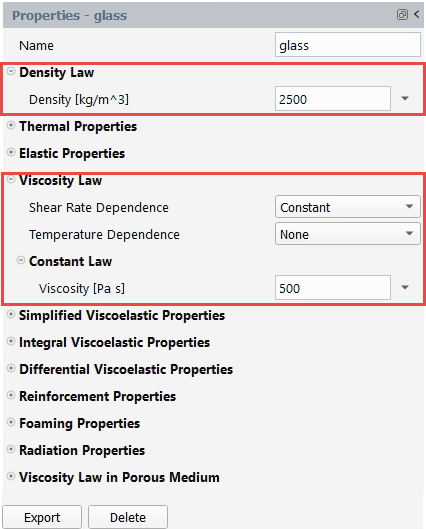
Enter glass for the Name.
Expand the Density Law and Viscosity Law categories.
In the Density Law category, enter
2500kg/m3 for the Density.In the Viscosity Law category, enter
500Pa s for the Viscosity.
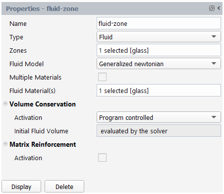
Define the cell zone properties for the fluid-zone.
Setup → Cell
Zones → fluid-zone
For Zones, select the field to open a selection dialog.
In the selection dialog, select glass and click OK to keep the selection and close the dialog.
Retain the default selection of Generalized newtonian for Fluid Model .
Define the cell zone properties for the fixed-mold.
Setup → Cell
Zones → fixed-mold
For Zones, select the field to open a selection dialog.
In the selection dialog, select mold and click OK to keep the selection and close the dialog.
Define the cell zone properties for the moving-mold.
Setup → Cell
Zones → moving-mold
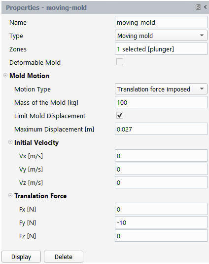
For Zones, select the field to open a selection dialog.
In the selection dialog, select plunger and click OK to keep the selection and close the dialog.
From the Motion Type drop-down list, select Translation force imposed.
Enter
100kg for Mass of the Mold.Enable the Limit Mold Displacement option.
Enter
0.027m for Maximum Displacement.Enter
-10N for Fy.
Set the conditions for the free-surface boundary.
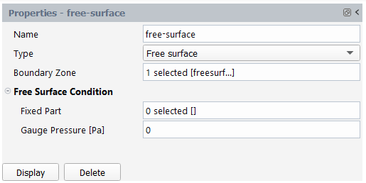
Select free-surface under Fluid Boundary Conditions in the Outline View to review this boundary condition for the simulation.
Select freesurface as the Boundary Zone.
Click Fluid Boundary Conditions in the Outline View, then click in the properties window.
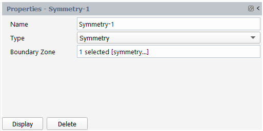
Enter Symmetry-1 for Name.
From the Type drop-down list, select Symmetry.
Select symmetry1 as the Boundary Zone.
Click Fluid Boundary Conditions in the outline view, then click in the properties window.
Enter Symmetry-2 for Name.
From the Type drop-down list, select Symmetry.
Select symmetry2 as the Boundary Zone.
Contact between the glass and the solid and moving molds can be accounted for using contact conditions.
Define the contact between the fluid zone and the fixed mold.
Under Contact Boundary Conditions, select contact-with-fixed-mold to edit the default properties of this contact condition for your simulation.
Select freesurface for the Fluid Zone of Contact.
Select moldcontact for the Mold Zone of Contact.
Enter
1e-4m for the Penetration Accuracy.
Define the contact between the fluid zone and the moving mold.
Under Contact Boundary Conditions, select contact-with-moving-mold to edit the default properties of this contact condition for your simulation.
Select freesurface for the Fluid Zone of Contact.
Select plungercontact for the Mold Zone of Contact.
Enter
1e-4m for the Penetration Accuracy.
Here, we will assign the glass to be a deforming fluid.
Under Mesh Deformations, select fluid-deformation to edit the default properties of the fluid deformation zone for your simulation.
Retain the selection of Lagrangian as the deformation Type.
Select glass for Zones.
Define the conditions and settings for adaptive meshing that will be used to refine the mesh during the solution.
Define the adaptive meshing condition (condition-1).
Setup → Adaptive
Meshing → Conditions →
condition-1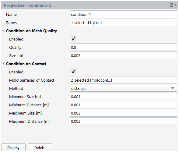
Select glass for Zones.
Select moldcontact and plungercontact for Mold Surfaces of Contact.
Select distance from the Method drop-down list.
Enter
0.001m for Minimum Size.Enter
0.001m for Minimum Distance.Enter
0.002m for Maximum Size.Enter
0.002m for Maximum Distance.
Edit the adaptive meshing properties.
Setup → Adaptive
Meshing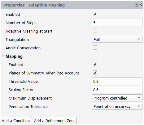
Enter
5for the Number of Steps.
Open the Solution branch of the Outline View (or use the Ribbon). Here, you can review problem setup and other solution properties. Most items indicate that current default values are appropriate.
Edit the Calculation Activities.
Solution → Calculation
Activities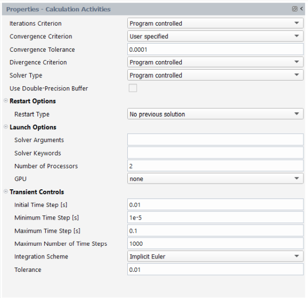
From the Convergence Criterion drop-down list, select User specified.
Enter
0.0001for the Convergence Tolerance.
Review your problem setup.
Solution → Run
CalculationClick Check to review your simulation settings. Fluent will inform you as to whether or not your setup contains any problems and will provide guidance to solve any issues.
Calculate a solution.
Click Calculate to start the calculation.
Click the Plots tab to view the plot of the convergence monitors.
Once the calculations are complete, check the solution's listing in the Transcript tab to confirm it's success. You can confirm that the solution proceeded as expected by looking for the following printed at the bottom of the listing file:
The computation succeeded.
Save the work.
Your work can be preserved using a "session" file - a Materials Processing workspace-specific case file (
*.mprcas) that contains your settings and your results.File → → , entering
glass_pressingas the name of the session
Review results using the various tools in the Results section of the Outline View or the Ribbon where you can setup contours, vectors, and so on.
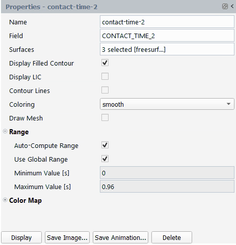
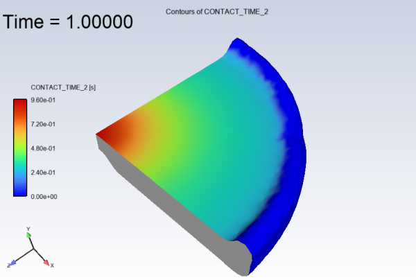
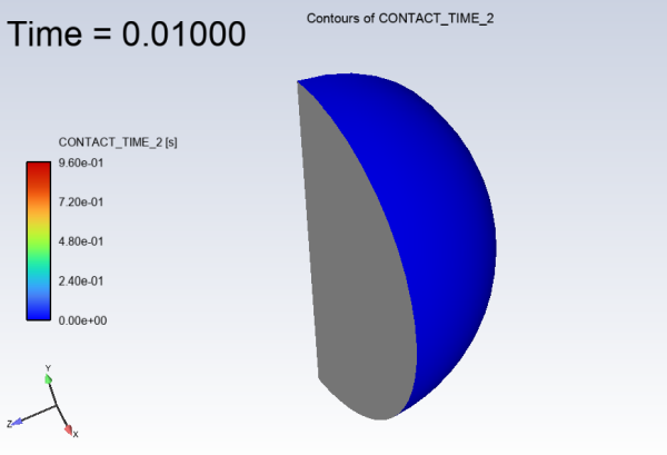
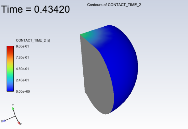
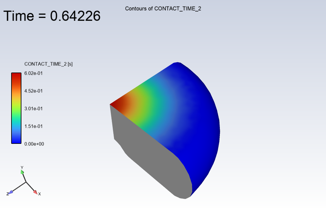
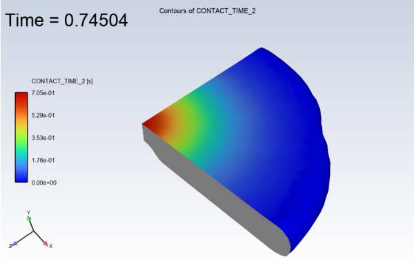
Display contours of contact time (CONTACT_TIME_2) for the freesurface, symmetry1, and symmetry2 surfaces.
The CONTACT_TIME_2 field corresponds with the length of time that the plunger is in contact with the fluid.
Results → Graphics
→ Contour → New Specify a new Name (
contact-time-2).For the Field, select CONTACT_TIME_2.
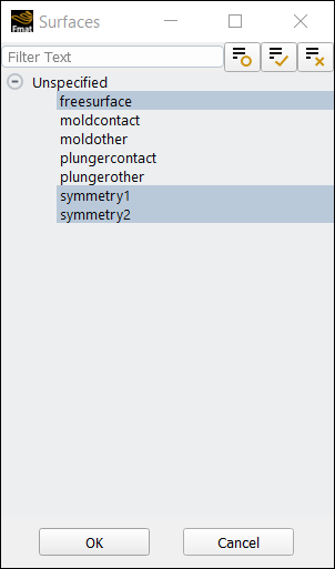
For the Surfaces, select the field to open the Surfaces dialog where you can select the relevant boundaries. Select freesurface, symmetry1, and symmetry2 from the list, and click OK to close the dialog.
For the contour properties, keep the remaining defaults and click Display to see the thickness contour plot in the graphics window.
Review an animation of the contour of CONTACT_TIME_2.
Results → Timestep
To reset the timesteps, change the Current animation time step value to
1. Alternatively, you can also move the slider all the way to the left, or click the Jump to Start button ( ).To start the animation, click the Play button (
) to start the
animation.To stop the animation, click the Stop button (
).
Display contours of initial coordinate y (COORDINI[Y]).
Results → Graphics
→ Contour → New Repeat the previous steps to create a new contour over the freesurface, symmetry1, and symmetry2 surfaces with the Name of
initial-coordinate-yand the Field set to COORDINI[Y].Repeat the previous steps to review an animation of the contour.
Display contours of initial coordinate x (COORDINI[X]).
Results → Graphics
→ Contour → New Repeat the previous steps to create a new contour over the freesurface, symmetry1, and symmetry2 surfaces, with Name of
initial-coordinate-x, Field set to COORDINI[X], and the Use Global Range option disabled.Repeat the previous steps to review an animation of the contour.
![Contours of Initial Coordinate Y (COORDINI[Y])](graphics/g_flu_tg_matpro_glass_coordiniy_contours.png)
![Contours of Initial Coordinate X (COORDINI[X])](graphics/g_flu_tg_matpro_glass_coordinix_contours.png)
This tutorial introduced the concept of a 3D pressing problem using the Fluent Materials Processing workspace. You solved the problem using a 3D geometry for the fixed mold and the plunger and made suitable assumptions about the physics of the problem. The plunger moves downward and presses the fluid against a fixed 3D mold to obtain the desired shape.
This tutorial is divided into the following sections:
This tutorial illustrates the simulation of an extrusion process with adaption of a die geometry to obtain the desired extrudate shape, using the Fluent Materials Processing workspace (Fluent Materials Processing Workspace).
In this tutorial you will learn how to use the Fluent Materials Processing workspace to:
Easily set up your inverse extrusion simulation.
Calculate a solution.
Analyze the results.
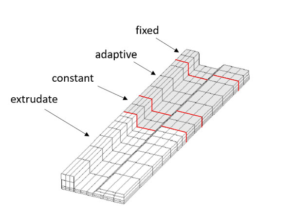
This tutorial covers the simulation of a non-isothermal extrusion process to predict the shape of a die for a given extrudate shape. The initial configuration of the die and extrudate geometry is shown in Figure 3.43: Problem Description, which consists of four distinct cell zones:
extrudate
Cell zone for the extrudate geometry.
constant
Cell zone for the constant portion of the die.
adaptive
Cell zone for the adaptive portion of the die.
fixed
Cell zone for the fixed portion of the die.
The extrudate cell zone contains the following boundaries:
extrudate-exit (Type = Extrudate exit). See Figure 3.44: Boundaries.
free-surface (Type = Free surface). See Figure 3.44: Boundaries.
The free-surface will be fixed to the wall-constant boundary (shown in Figure 3.45: Constant, Adaptive, and Fixed Walls) by means of a Free Surface Condition.
guide (Type = Wall). See Figure 3.46: Extrudate Guide.
symmetry-extrudate (Type = Symmetry). See Figure 3.47: Symmetries.
The constant cell zone contains the following boundaries:
wall-constant (Type = Wall). See Figure 3.45: Constant, Adaptive, and Fixed Walls.
symmetry-constant (Type = Symmetry). See Figure 3.47: Symmetries.
The adaptive cell zone contains the following boundaries:
wall-adaptive (Type = Wall). See Figure 3.45: Constant, Adaptive, and Fixed Walls.
symmetry-adaptive (Type = Symmetry). See Figure 3.47: Symmetries.
The fixed cell zone contains the following boundaries:
wall-fixed (Type = Wall). See Figure 3.45: Constant, Adaptive, and Fixed Walls.
symmetry-fixed (Type = Symmetry). See Figure 3.47: Symmetries.
inlet (Type = Inflow). See Figure 3.44: Boundaries.
The figures below show the relevant boundaries for the extrudate, constant, adaptive, and fixed cell zones.
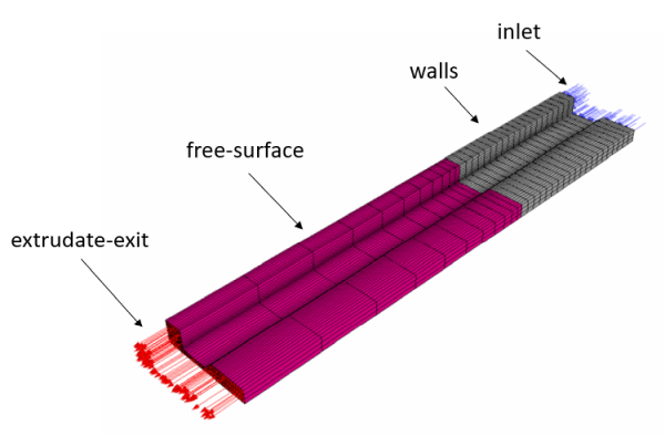
Figure 3.44: Boundaries shows the free-surface displayed in pink and the extrudate-exit and inlet displayed with red arrows and blue arrows, respectively. Note that walls (displayed in gray) consists of the wall-constant, wall-adaptive, and wall-fixed boundaries.
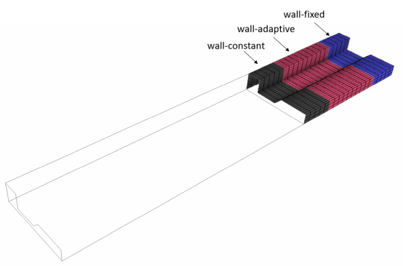
Figure 3.45: Constant, Adaptive, and Fixed Walls shows boundaries wall-constant, wall-adaptive, and wall-fixed.
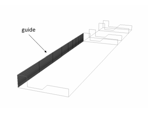
Figure 3.46: Extrudate Guide shows the guide within the extrudate cell zone.
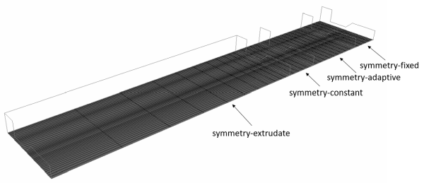
Figure 3.47: Symmetries shows the boundaries that support a symmetry condition: symmetry-extrudate, symmetry-constant, symmetry-adaptive, and symmetry-fixed.
Convergence can be difficult to achieve when computing inverse extrusion problems, especially for non-isothermal cases. However, the Fluent Materials Processing workspace is equipped with convergence strategies for handling such difficulties. The appropriate convergence strategies are activated automatically by the wizard, used in this tutorial.
The following sections describe the setup and solution steps for this tutorial:
To prepare for running this tutorial:
Prepare a working folder for your simulation.
Download the
inverse_extrusion.zipfile here .Unzip the
inverse_extrusion.zipfile you have downloaded to your working folder.The polyflow mesh file
invext.polycan be found in the unzipped folder.
Use the Fluent Launcher to start Ansys Fluent.
Select Materials Processing in the list of Fluent workspaces.
Click Start.
Clicking Start in the Fluent Launcher opens the Fluent Materials Processing workspace.
The workspace is a version of Ansys Fluent that utilizes the power of the Ansys Polyflow solver to simulate polymer flows such as extrusion, blow molding, pressing, and so forth.
Open an extrusion geometry by reading in a Polyflow mesh file.
In the Setup properties, under Read, click the Mesh... button.
You can also use the File menu, and choose Read > Polyflow Mesh....
Locate and select the polyflow mesh file from your working folder (
invext.poly).
Use the wizard to set up an inverse extrusion simulation (using the Simulation category of the Setup Ribbon).
Setup
→ Simulation → Use
Wizard...
This will display the Wizard dialog.
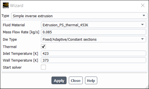
Set the Type to Simple inverse extrusion.
For Fluid Material select Extrusion_PS_thermal_453K.
Enter
0.085kg/s for the Mass Flow Rate.For Die Type select Fixed/Adaptive/Constant Sections.
Enable the Thermal option.
Enter
423K and373K for the Inlet Temperature and Wall Temperature, respectively.Click Apply.
This will instruct the workspace to set up the appropriate objects and settings based on your selections.
Note: Notice the Outline View's use of status icons. A green check mark indicates the properties of that object are satisfactory. A red 'x' indicates that attention is required for that object.
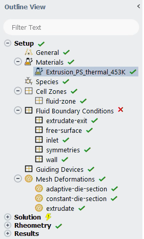
You can progress down the Outline View (or across the Ribbon) to complete your simulation settings using each object's property pages.
Click the General node in the Outline View to display general settings for the problem setup.
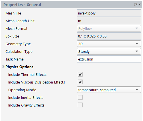
Select General in the Outline View to review general properties of the simulation.
Review the settings in the properties page.
In the following steps you will set the conditions at each of the boundaries of the simulation.
Set the free surface conditions.
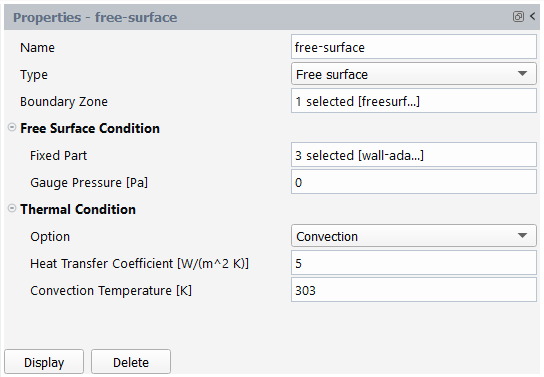
Select free-surface under Fluid Boundary Conditions in the Outline View to review free surface boundary conditions for the simulation.
Select Convection for the thermal condition Option.
Enter
5W/(m2K) for the Heat Transfer Coefficient.Enter
303K for the Convection Temperature.
Set the wall conditions.
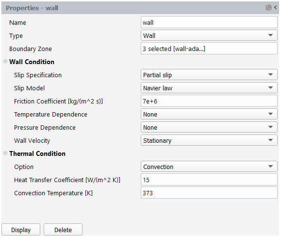
Select wall under Fluid Boundary Conditions in the Outline View to review wall boundary conditions for the simulation.
Select Partial Slip for Slip Specification as the Boundary Zone.
Enter
7e6kg/(m2s) for the Friction Coefficient.Select Convection for the thermal condition Option.
Enter
15W/(m2K) for the Heat Transfer Coefficient.Enter
373K for the Convection Temperature.
Create the boundary condition for the guide.
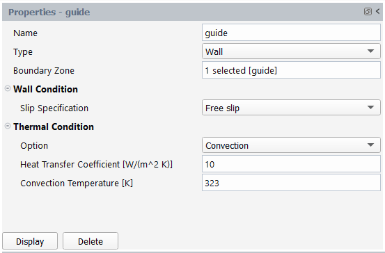
Select Fluid Boundary Conditions in the Outline View, and click the New... button in the properties window, or right-click in the tree and add a new condition to the tree.
Rename the new condition to guide.
Set the Type to Wall.
Select guide as the Boundary Zone.
Select Free slip for Slip Specification.
Select Convection for the thermal condition Option.
Enter
10W/(m2K) for the Heat Transfer Coefficient.Enter
323K for the Convection Temperature.
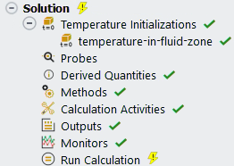
Open the Solution branch of the Outline View (or use the Ribbon). Here, you can review problem setup and other solution properties. Most items indicate that current default values are appropriate.
Review your problem setup.
Select Run Calculation to see available options.
Click Check to review your simulation settings. The workspace will inform you as to whether or not your setup contains any problems and will provide guidance to solve any issues.
Calculate a solution.
Click Calculate to start the calculation.
Click the Plots tab to view the plot of the convergence monitors.
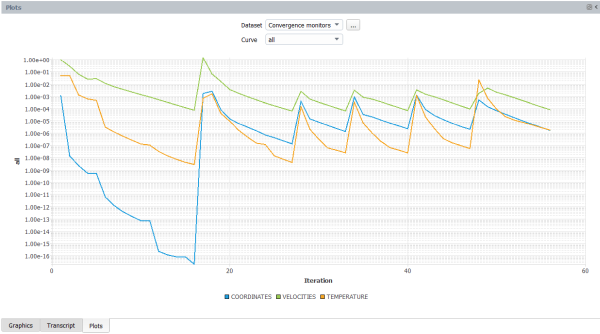
Once the calculations are complete, check the solution's listing in the Transcript tab to confirm its success. You can confirm that the solution proceeded as expected by looking for the following printed at the bottom of the listing file:
The computation succeeded.
Save the work.
Your work can be preserved using a "session" file - a Materials Processing workspace-specific case file (
*.mprcas) that contains your settings and your results.File → → , entering
inverse_extrusionas the name of the session.
Review results using the various tools in the Results section of the Outline View or the Ribbon where you can setup contours, vectors, and so on.
Click the Graphics tab to display the graphics window.
Display an isometric view of the geometry by clicking the
 button in the graphics toolbar, then select
Isometric from the drop-down.
button in the graphics toolbar, then select
Isometric from the drop-down.Display the velocity distribution for the fluid zone.
Results → Quick-View
→ Velocity
→ fluid-zoneRepeat the previous step to create a Pressure contour for the fluid zone using the Quick-View in the ribbon.
Repeat the previous steps to create a Temperature contour for the fluid zone using the Quick-View in the ribbon.
The temperature plot shows that the temperature of the fluid has increased due to viscous dissipation. Additionally, heat exchange with the wall has caused the fluid to cool in the corners of the channel.
Display the geometry from the +Y direction by clicking the
button in the graphics toolbar, then select From
+Y Direction from the drop-down.From the +Y direction, the deformation of the die and the free jet can be seen.
Display the geometry from the +Z direction by clicking the
button in the graphics toolbar, then select From
+Z Direction from the drop-down.Display contours of velocity magnitude for the die lip.
Results → Graphics
→ Contour → New Enter Die_lip for Name.
For the Field, select VELOCITIES[].
For Surfaces, select the field to open the Surfaces dialog where you can select the relevant boundaries. Select extrudate-constant from the list and click OK to close the dialog.
Click the button in the properties panel to view the die lip.
In the properties panel, enable Draw Mesh, then select Mesh Outline from the Overlayed Mesh drop-down.
Click Display.
Use the Graphics window to adjust the view as shown in the following figure.
The plot shows that the left part of the die has been enlarged and the right part has been reduced, relative to the extrudate shape. This is due to the slower fluid velocity in the left portion of the die and higher fluid velocity in the right portion. Additionally, the fluid in the left portion of the die is accelerated leading to the geometry reduction, while the fluid in the right portion of the die is slowed leading to geometry enlargement.
Create a YZ plane for observing the fluid velocity in the left portion of the die.
Results → Surfaces
→ Plane → New 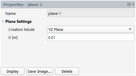
Select YZ Plane for Creation Mode.
Enter
0.01m for X.
Create an additional YZ plane for observing the fluid velocity in the right portion of the die.
Select YZ Plane for Creation Mode.
Enter
0.075m for X.
Display contours of velocity to observe the fluid velocity in the left portion of the die.
Results → Graphics
→ Contour → New Enter velocity-left-block for Name.
For the Field, select VELOCITIES[Z].
For the Surfaces, select plane-1.
Click Display.
View the geometry from the +X direction by clicking the
button in the graphics toolbar, then select
From +X Direction from the drop-down.
Display contours of velocity to observe the fluid velocity in the right portion of the die.
Results → Graphics
→ Contour → New Enter velocity-right-block for Name.
For the Field, select VELOCITIES[Z].
For the Surfaces, select plane-2.
Click .
Create a line surface for the left portion of the die.
Results → Surfaces
→ Line → New Set First Points as
0.01,0.0125, and-0.2m for X, Y, and Z, respectively.Set Second Points as
0.01,0.0125, and0.35m for X, Y, and Z, respectively.
Repeat the previous procedure to create a line surface for the right portion of the die, by entering
0.075,0.005,-0.2,0.075,0.005, and0.35for First Point X, First Point Y, First Point Z, Second Point X, Second Point Y, and Second Point Z, respectively.Create an XY plot to observe the fluid acceleration in the left and right portions of the die.
Results → Plots
→ XY Plot → New
Select line-1 and line-2 for Lines.
Select Velocities[Z] for the Field.
Set the Plot Direction as
0,0, and1for X Component, Y Component, and Z Component, respectively.Expand the Curves category and select - - - - from the Pattern drop-down list.
Select * from the Symbol drop-down list, then enter
0.4for the Size.Click Plot.
From the plot it can be seen that the fluid accelerates in the extrudate along line-1 (corresponding to the left block of the die), while the fluid slows down in the extrudate along line-2 (corresponding to the right block of the die).
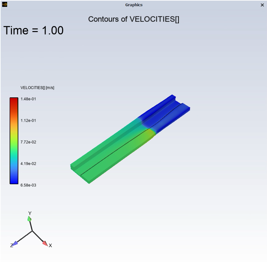
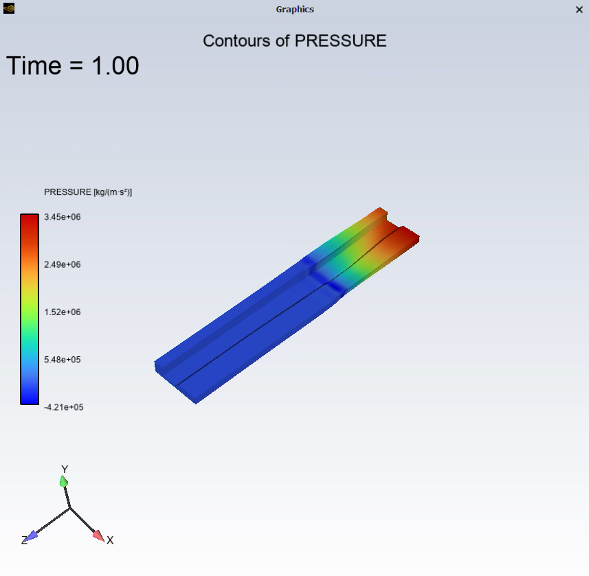
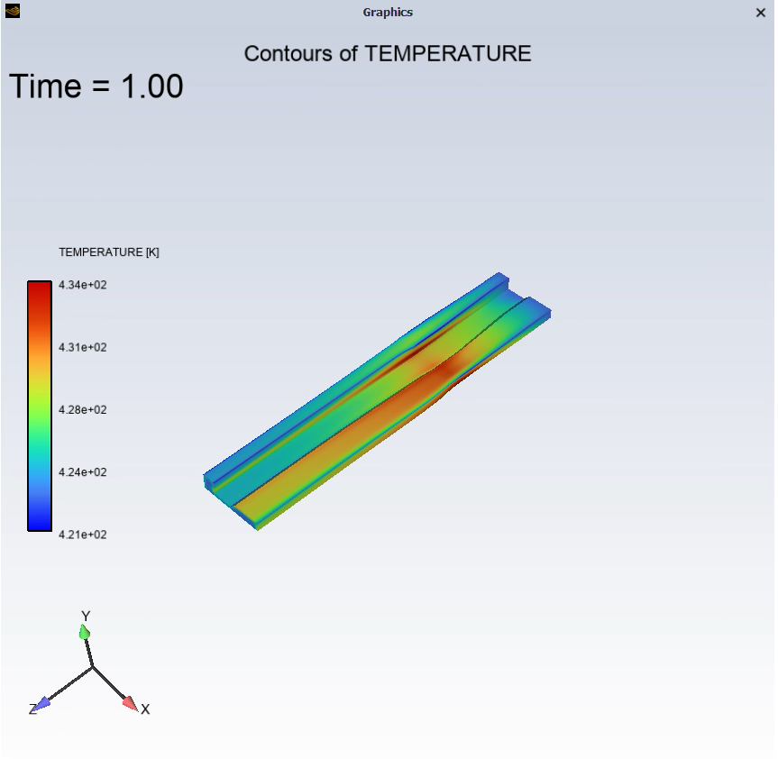
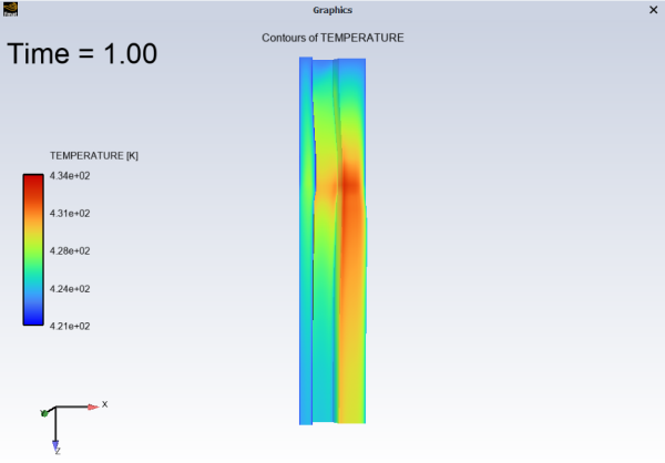
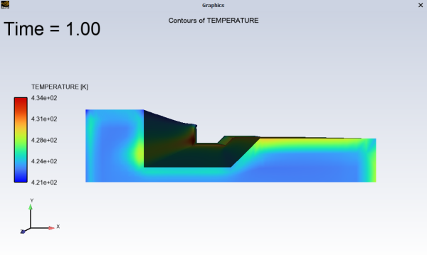
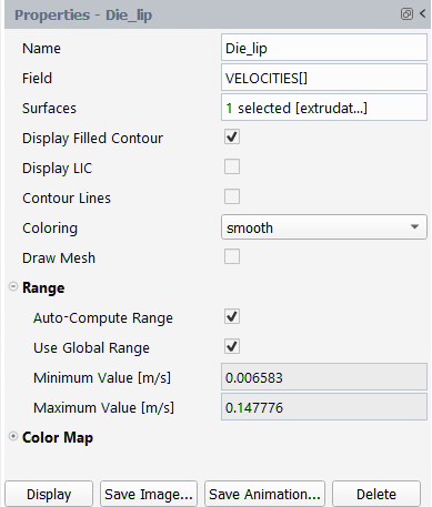
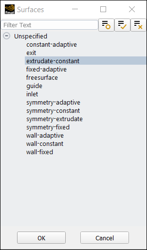
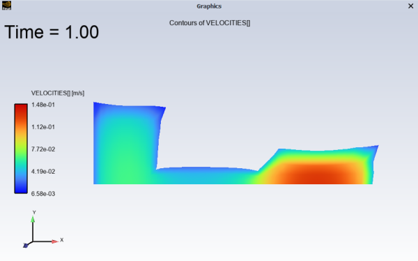
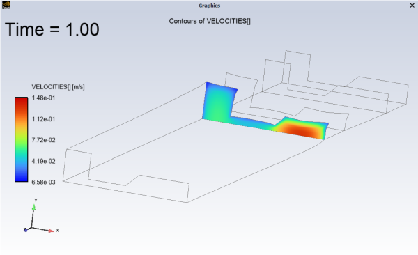
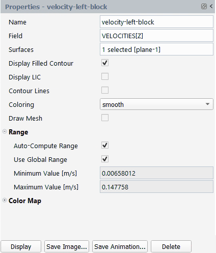
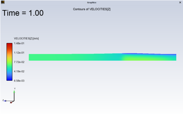
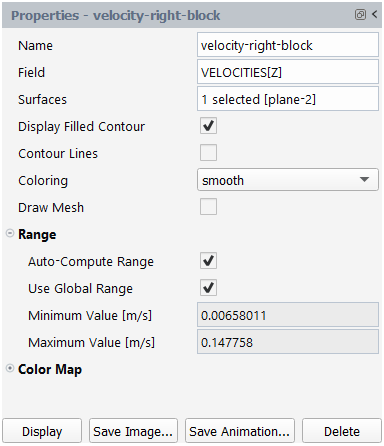
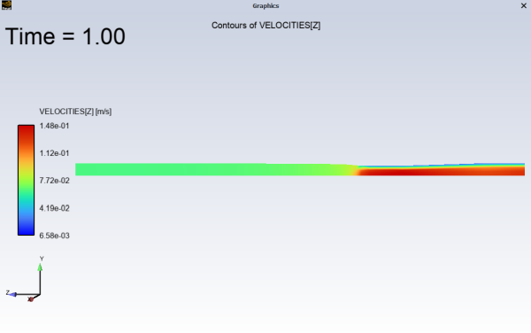
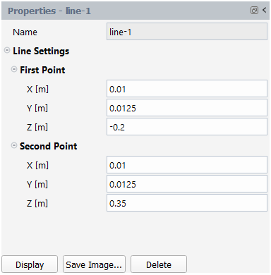
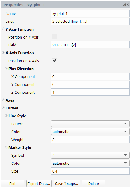
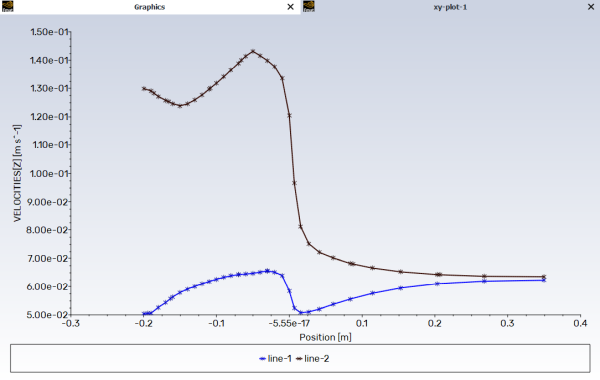
This tutorial introduced the concept of a 3D inverse extrusion problem using the Fluent Materials Processing workspace. You solved the problem using a simple geometry for the extrudate, made suitable assumptions about the physics of the problem, and analyzed the factors affecting the predicted die shape.
This tutorial is divided into the following sections:
This tutorial describes how to use the mesh superposition technique within the Fluent Materials Processing workspace (Fluent Materials Processing Workspace).
In this tutorial you will learn how to use the Fluent Materials Processing workspace to:
Easily set up your simulation using the mesh superposition technique.
Calculate the solution.
Analyze the results and generate a scene of the fluid temperature distribution.
This tutorial demonstrates the use of the mesh superposition technique in the Fluent Materials Processing workspace to analyze the flow of a non-isothermal fluid through a single rotating screw extrusion device.
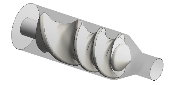
The flow domain consists of an extruder wall, screw, screw shaft, one inlet, and one outlet. These components are shown below in Figure 3.65: Flow Domain Components. For the purpose of this description, a clipped surface of the extruder wall is displayed.
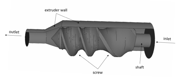
The fluid enters into the extruder through an inlet shown below in Figure 3.66: Extruder Boundaries at a volume flow rate of Q = 3 * 10-5 m3 / s, before encountering the solid steel rotating screw. The fluid has the following material properties:
Viscosity: Bird-Carreau

with,
Density = 1200 kg / m3
Thermal conductivity = 1 W / m / K
Heat capacity (Cp) = 1700 J / kg / K


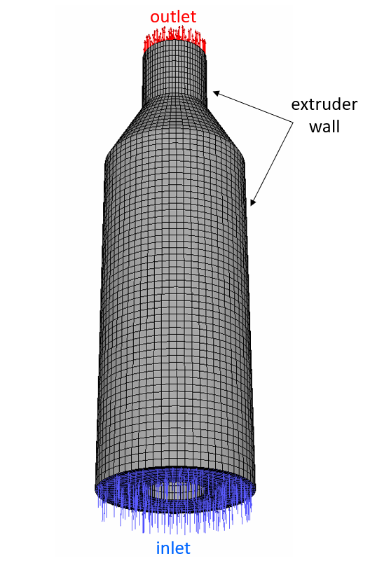
For simplicity, the screw is defined as an overlapping part by use of the mesh superposition technique. The mesh of the flow domain can be seen below in Figure 3.67: Mesh of the Flow Domain.
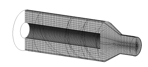
All nodes of the flow domain inside the screw will be constrained and their velocity will be imposed. The density, thermal conductivity, and heat capacity for solid steel will be applied on nodes of the flow domain that overlap with the screw, which is shown below in Figure 3.68: Screw Mesh.
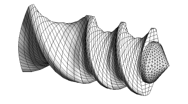
The following sections describe the setup and solution steps for this tutorial:
To prepare for running this tutorial:
Download the
SSE_thermal.zipfile here .Unzip
SSE_thermal.zipto your working directory.The file,
sse_thermal.mshcan be found in the folder.
Use the to start Ansys Fluent.
In the Fluent Launcher, set the Capability Level to Enterprise.
The mesh superposition technique (MST) in the Fluent Materials Processing workspace is only available with the Enterprise licensing level.
Select Materials Processing in the list of Fluent workspaces.
Click Start.
Clicking Start in the Fluent Launcher opens the Fluent Materials Processing workspace.
Load the provided mesh file.
In the Setup properties, under Read, click the Mesh... button.
You can also use the File menu, and choose Read > Polyflow Mesh....
Locate and select the mesh file from your working folder (
sse_thermal.msh).Set the Mesh Length Unit to mm, and click to close the dialog box.
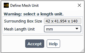
Set up an extrusion simulation (using the Simulation category of the Setup Ribbon).
Setup → Simulation
→ Use Template...
This will display the Simulation Template dialog.
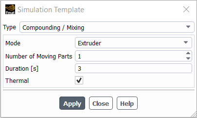
Set the Type to Compounding / Mixing.
Set the Mode to Extruder.
Set the Number of Moving Parts to 1.
Set the Duration to 3 seconds.
Enable the Thermal option.
Click Apply.
This will instruct the workspace to set up the appropriate objects and settings based on your selections.
Note: Notice the Outline View's use of status icons. A green check mark indicates the properties of that object are satisfactory. A red 'x' indicates that attention is required for that object.
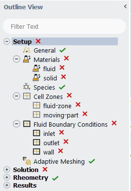
You can progress down the Outline View (or across the Ribbon) to complete your simulation settings using each object's property pages.
Click the General node in the Outline View to display general settings for the problem setup. For this tutorial, you can keep the default settings.
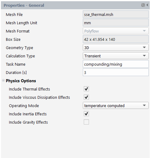
Edit the density and viscosity settings for the fluid material.
Setup →
Materials → fluid
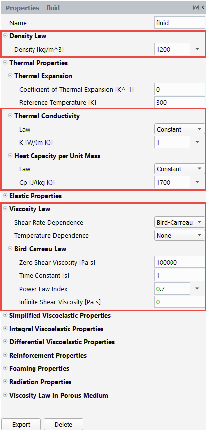
Expand the Density Law category.
Enter
1200kg/m3 for the Density.
Expand the Thermal Properties category.
Under Thermal Conductivity, enter
1W/(m K) for K.Under Heat Capacity per Unit Mass, enter
1700J/(kg K) for Cp.
Expand the Viscosity Law category.
Select Bird-Carreau from the Shear Rate Dependence drop-down list.
Under Bird-Carreau Law, enter
100000Pa s for Zero Shear Viscosity,1s for Time Constant, and0.7for the Power Law Index.
Import a new material for the screw.
Click the Import from library button in the Materials property page. Alternatively, you can right-click on the Materials node, and select Import from library from the context menu.
Materials Import from
library 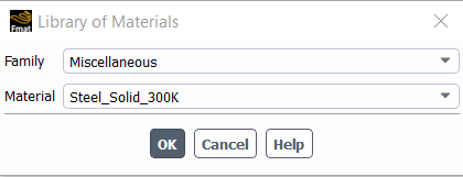
Select Miscellaneous for the Family
Select Steel_Solid_300K for the Material.
Click OK to close the dialog.
The new material will be added to the list of materials in the Outline View.
Remove the original solid material solid.
Select solid in the Outline View, right-click and select Delete from the context menu.
Setup →
Materials → solid
Delete
You will be prompted to make sure you want to remove the material. Click Yes to remove the material.
In this portion of the tutorial, you will assign the fluid and moving part cell zones.
Define the cell zone properties for the fluid-zone.
Setup → Cell
Zones → fluid-zone
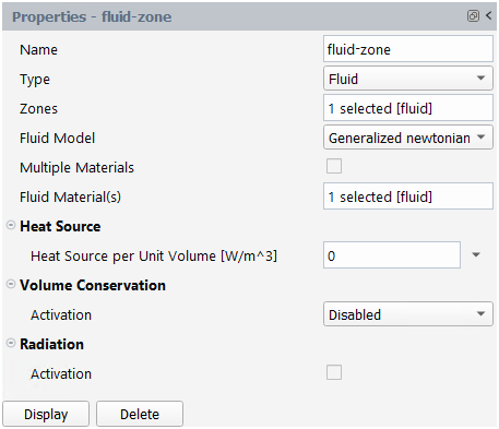
For Zones, select the field to open a selection dialog.
In the selection dialog, select fluid and click OK to keep the selection and close the dialog.
Retain the default selection of Generalized newtonian for Fluid Model .
Define the cell zone properties for the moving-part.
Setup → Cell
Zones → moving-part
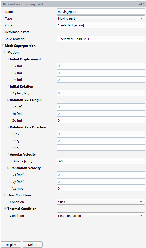
For Zones, select screw.
For the Solid Material, select Solid Steel.
Under Angular Velocity, enter
-60rpm for Omega.
Set the conditions for the inlet boundary.
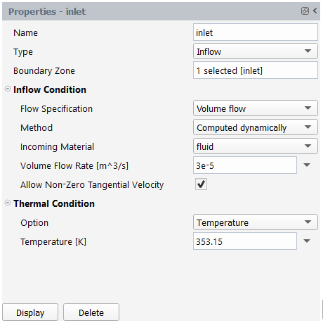
Select inlet under Fluid Boundary Conditions in the Outline View.
Select Volume flow for the Flow Specification.
For the Method, select Computed dynamically.
Due to the rotation of the extruder wall, computed dynamically is specified for the inflow condition, which will search the normal force to the inlet that must be set in order to obtain the prescribed volumetric flow rate.
For the Volume Flow Rate, enter
3e-5m3/s.Under Thermal Condition, enter
353.15K for the Temperature.
Set the conditions for the outlet boundary.
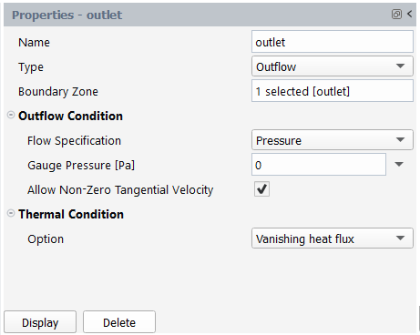
Select outlet under Fluid Boundary Conditions in the Outline View.
Select outlet for the Boundary Zone.
Set the conditions for the wall boundary.
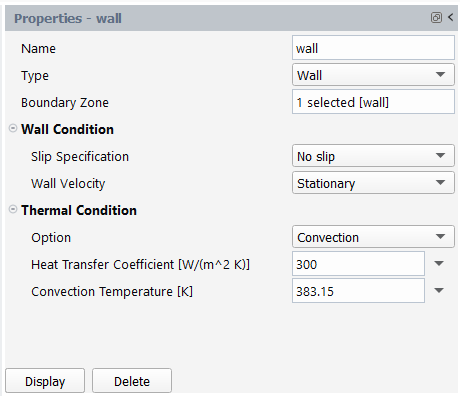
Select wall under Fluid Boundary Conditions in the Outline View.
Select wall for the Boundary Zone.
Under Thermal Condition, select Convection for the Option.
Enter
300W/(m2 K) for the Heat Transfer Coefficient.Enter
383.15K for the Convection Temperature.
Create a new boundary condition for the screw shaft.
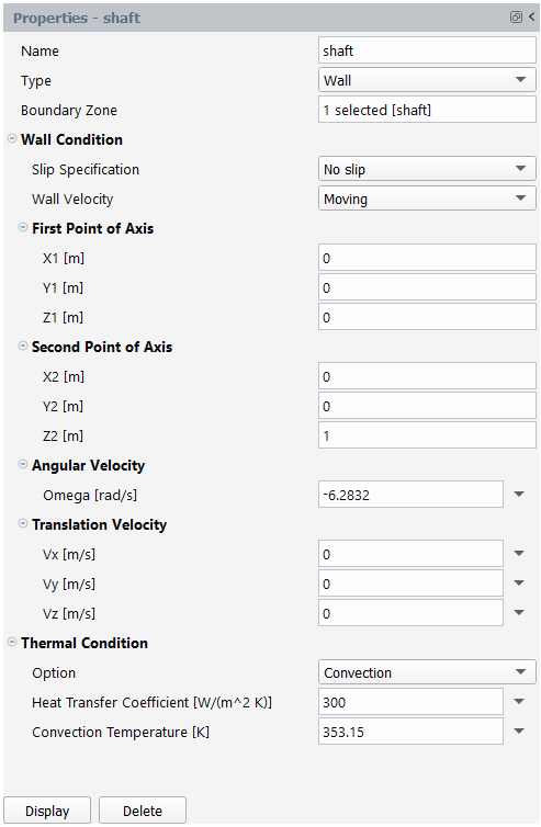
Click Fluid Boundary Conditions in the outline view, then click in the properties window.
Enter shaft for the Name.
From the Type drop-down list, select Wall.
Select shaft as the Boundary Zone.
Select Moving for the Wall Velocity.
Under First Point of Axis, enter
0m for X1,0m for Y1, and0m for Z1.Under Second Point of Axis, enter
0m for X2,0m for Y2, and1m for Z2.Under Angular Velocity, enter
-6.2832rad/s for Omega.Although the shaft is rotating at the same angular velocity as the screw, the units of angular velocity for rotating walls is specified in rpm while rad/s is used for moving parts.
Under Translation Velocity, enter
0m/s for Vx,0m/s for Vy, and0m/s for Vz.Under Thermal Condition, select Convection for the Option.
Enter
300W/(m2 K) for the Heat Transfer Coefficient.Enter
353.15K for the Convection Temperature.
Open the Solution branch of the Outline View (or use the Ribbon). Here, you can review problem setup and other solution properties. Most items indicate that current default values are appropriate.
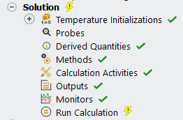
Set the Temperature Initializations.
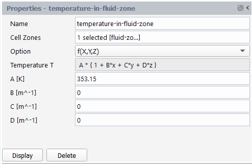
Click temperature-in-fluid-zone under Temperature Initialization in the Outline View.
Enter
353.15K for A.
Edit the solution Methods.
Solution →
Methods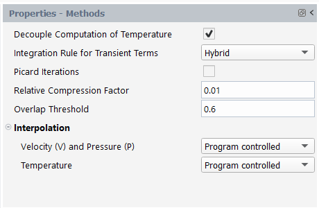
Enable the Decouple Computation of Temperature option.
Select Hybrid for Integration Rule for Transient Terms.
Edit the Calculation Activities.
Solution → Calculation
Activities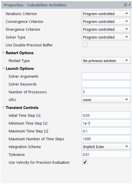
Under Launch Options, enter
5for the Number of Processors.Under Transient Controls, enter
0.05s for the Initial Time Step.
Edit the solution Outputs.
Solution →
Outputs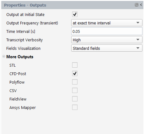
Enter
0.05s for the Time Interval.
Review your problem setup.
Solution → Run
CalculationClick Check to review your simulation settings. The workspace will inform you as to whether or not your setup contains any problems and will provide guidance to solve any issues.
Calculate a solution.
Click Calculate to start the calculation.
Click the Plots tab to view the plot of the convergence monitors.
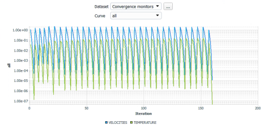
Once the calculations are complete, check the solution's listing in the Transcript tab to confirm it's success. You can confirm that the solution proceeded as expected by looking for the following printed at the bottom of the listing file:
The computation succeeded.
Save the work.
Your work can be preserved using a "session" file - a Materials Processing workspace-specific case file (
*.mprcas) that contains your settings and your results.File → → , entering
sse_thermalas the name of the session
Review results using the various tools in the Results section of the Outline View or the Ribbon where you can create new surfaces, setup contours, and create scenes.
Display the temperature distribution on the inlet, outlet, and extruder wall.
Results → Graphics
→ Contour → New Enter
temperaturefor the Name.For the Field, select TEMPERATURE.
For the Surfaces, select the field to open the Surfaces dialog where you can select the relevant boundaries. Select inlet, outlet, and wall from the list, then click OK to close the dialog.
For the contour properties, keep the remaining defaults and click Display to see the temperature contour plot in the graphics window.
In the following steps, you will create new surfaces for displaying the temperature field, which will then be used to create a scene.
Create a new iso-surface on the domain.
Results → Sufaces
New →
Iso-Surface...
Enter
x=0for the Name.For the Field, select Coordinates[X].
For Iso-Value, enter
0m.
Create a new iso-clip for one half of the extruder wall.
Results → Sufaces
New →
Iso-Clip...
Enter
x<0for the Name.For the Field, select Coordinates[X].
From the Surfaces list, select wall.
Enter
-0.021m for the Minimum.Enter
0m for the Maximum.
Repeat the previous step to create another iso-clip for the second half of the wall surface, with the Name of
x>0, the Minimum set to0m, and the Maximum set to0.021m.Display the temperature distribution on the second half of the flow domain.
Results → Graphics
→ Contour → New Enter
temperature-x-greater-than-0for the Name.For the Field, select TEMPERATURE.
For the Surfaces, select the field to open the Surfaces dialog where you can select the relevant boundaries. Select x>0, x=0, inlet, and outlet from the list, then click OK to close the dialog.
Deselect the Auto-Compute Range option.
Enter
350K and440K for the Minimum Value and Maximum Value, respectively.Expand the Color Map category.
Enter
100for the Color Map Size.From the Type list, select float.
Enter
0for the Precision.Disable the Automatically Skip Labels option, then enter
11for Skip.Click Display to see the temperature contour plot in the graphics window.
Repeat the previous step to create an additional contour plot for the other half of the extruder wall, with the Name of
temperature-x-less-than-0and only x<0 selected for Surfaces.Create a new mesh object for the screw.
Results → Meshes
New...
Enter
screwfor the Name.From the Surfaces list, select screwsurf and shaft.
Disable the Edges option.
Using the newly created graphics objects, create a scene of the temperature field.
Results → Scenes
New...
Deselect any objects that are enabled by default within the list of Graphics Objects.
Under the deformed category in the list of Graphics Objects, enable screw, temperature-x-greater-than-0, and temperature-x-less-than-0.
For temperature-x-less-than-0, set the Transparency to
80.Click to view the scene in the Graphics window.
Play the animation for the new scene.
Results → Timestep
To reset the timesteps, change the Current animation timestep value to
1. Alternatively, you can also move the slider all the way to the left, or click the Jump to Start button ( ).To start the animation, click the Play button (
).To stop the animation, click the Stop button (
).
The results displayed above show that the extruder wall and the screw experience the greatest temperature rise and the temperature within the flow domain increases from inlet to outlet due to the generated heat. The heat is generated almost exclusively within the thin layer adjacent to the barrel wall, and it appears that the screw is the primary source heating the main stream of fluid.