


The Fluent Materials Processing workspace is a means to explore manufacturing applications of highly viscous materials such as polymer extrusion, blowmolding, fiber spinning, etc. within the Fluent environment. Many of the models and concepts in this workspace are based onFluent Materials Processing, details of which can be found in the Fluent Materials Processing documentation (Polyflow User's Guide).
The Fluent Materials Processing workspace is a finite-element program primarily designed for the analysis of industrial flow processes dominated by nonlinear viscous phenomena and viscoelastic effects under various conditions. The work environment provides an easy access to most of the features available intoFluent Materials Processing software of which it is the successor.
The Fluent Materials Processing workspace is used in a wide variety of applications, including polymer and rubber processing, food rheology, glass pressing, and many other cases involving the flow of non-Newtonian fluids. These several applications, steady or transient, are essentially described by means of appropriate geometry, material models and suitable boundary conditions, and can be combined with thermal effects.
Geometry
The Fluent Materials Processing workspace allows you to setup both 2D, 3D and shell cases, where the geometric context is specified by providing a finite element mesh with the required dimension. Providing a 2D mesh in the XY-plane enables several possibilities. Indeed, next to the usual 2D planar and 2D axisymmetric cases, a 2D mesh can also be the geometric support for 2D channel and swirling cases, that is, cases involving three velocity components depending on two space variables. If the workspace detects a surface in the space, a (transient) shell model will be activated.
Rheology - Fluid Properties
In terms of fluid models, the theoretical foundation of the workspace is provided by the general principles of continuum mechanics, together with phenomenological or kinetic theoretical models for describing the rheological behaviour of the fluid. More precisely, processed materials are usually characterised by shear-thinning, and it is often the primary property to be considered. Other properties may develop, and they may have a more or less visible effect on the flow, depending on the context; one may mention here the first normal stress difference which develops in shear flows, the elongation viscosity, which develops in stretching deformations, and whose visible consequence is often strain hardening. For describing these properties, a relatively broad spectrum of fluid models is available in the workspace, and encompasses the generalized Newtonian inelastic fluid models as well as viscoelastic models.
Summarily, the generalized Newtonian inelastic models are available for all applications; differential viscoelastic models as well as the simplified viscoelastic model are available for 2D and 3D cases, but do not support support flows with restrictors; eventually integral viscoelastic models are available for blow moulding and thermoforming applications when the shell model is involved. At this level, you have the opportunity to read a material file from a library of fluid models, or to specify your own material and possibly to save it into a local library of material data files.
In addition, there are a few other flow models, such as foaming, coextrusion, or reinforcements, etc. that are introduced in the appropriate sections.
Heat Transfer
All setups can also be defined under thermal conditions. In this case, thermal properties will also be specified, as well as temperature dependence of fluid properties. Conjugated heat transfer between fluid and the fixed or moving solid can also be calculated.
Boundary Conditions
In terms of boundary conditions, the workspace offers a broad spectrum of possibilities, enabling the description of several applications. For fluid flows, the most typical boundary conditions are inlets, outlets, fixed or moving walls with or without slipping along the wall, free surfaces, plane of symmetry.
Under thermal conditions, thermal boundary conditions such as assigned temperature or heat flux can be imposed.
Convergence Strategies
When modeling industrial flows of rheologically complex materials, you often face non-linearities that have multiple origins. The most often encountered non-linearities originate from:
the rheology with the dependence of properties with respect to the local kinematic,
the thermal effects with viscous heating and transport of temperature, and
the free surface boundary condition that dictates the deformation of an extrudate and leads to an interaction between velocity and shape.
Other sources of non-linearities do exist, while you should note that these many non-linearities are often combined.
Handling non-linearities is often challenging. Hence, for facilitating the setup and for allowing you to focus on the flow model, convergence strategies are made available. You simply have to enable them as appropriate. Application-specific usage of such strategies is provided in the corresponding sections.
All these components, geometry, material model, boundary conditions, define a given application. The Fluent Materials Processing workspace is purposely designed to take these components and to assist you in setting up a simulation. The sections below describe the different applications that can be set up with the workspace and also specifies the context and the limitations.
The workspace supports the following features:
Extrusion / Coextrusion / Fiber spinning
Blow Molding / Thermoforming
Pressing / Forming
Film Casting
Filling
The supported geometry types include:
2D planar, 2D axisymmetric, 2D channel, 2D swirl, and 2D film
Shell
3D
The supported model attributes include the following:
Generalized Newtonian (isothermal & thermal)
Viscoelasticity
Foaming
The supported solver attributes include the following:
Steady-state
Time-dependent / Transient
Continuation
The Fluent Materials Processing workspace requires the following components.
CFD-Enterprise, CFD-Premium, or CFD-Pro license
Ansys Polyflow
Ansys EnSight
A valid
%HOME%environment variable assignment
Fluent Materials Processing is available at three different licensing levels, controlling the availability of various features and functionalities:
Enterprise—full access to all capabilities (along with those CFD Premium and CFD Pro features), including:
Mesh Superposition Technique (MST)
Volume of Fluid (VOF)
Filling
Viscoelasticity & all material models with yield stress
Porous media
2D & 3D contact
Premium—full access to the following capabilities:
Extrusion/coextrusion (interface and species)
Blow molding
Thermoforming
Film Casting
Constant viscosity and generalized non-Newtonian models (excludes Bingham, modified Bingham, Herschel-Bulkley, modified Herschel-Bulkley)
Link to Mechanical
Temperature
Material fitting
Shell contact
Starting from initial results
Free surface boundary conditions
Pro—(equivalent to Premium)
Note: The following limitations are known for the Fluent Materials Processing workspace:
Foaming cannot be combined with multiple materials and/or transport of species and/or generalized expressions defined on material properties.
If an expression is defined on density, you cannot impose a mass flow rate at the inlets and/or the outlets.
When using a limited Academic License, you cannot load a mesh containing more than 1,000,000 elements.
The graphical user interface (GUI) of Fluent Materials Processing is very similar to the solution mode of Fluent, in that:
it includes a ribbon, an outline view, a graphics window, a console, toolbars, dialog boxes, and quick search (as described in GUI Components in the Fluent User's Guide).
it can be modified (as described in Customizing the Graphical User Interface in the Fluent User's Guide).
it can be set to match your preferences (as described in Setting User Preferences/Options in the Fluent User's Guide). Preferences specific to the Fluent Materials Processing workspace are described in Setting Preferences for Fluent Materials Processing.
it has access to the help system (as described in Using the Help System in the Fluent User's Guide).
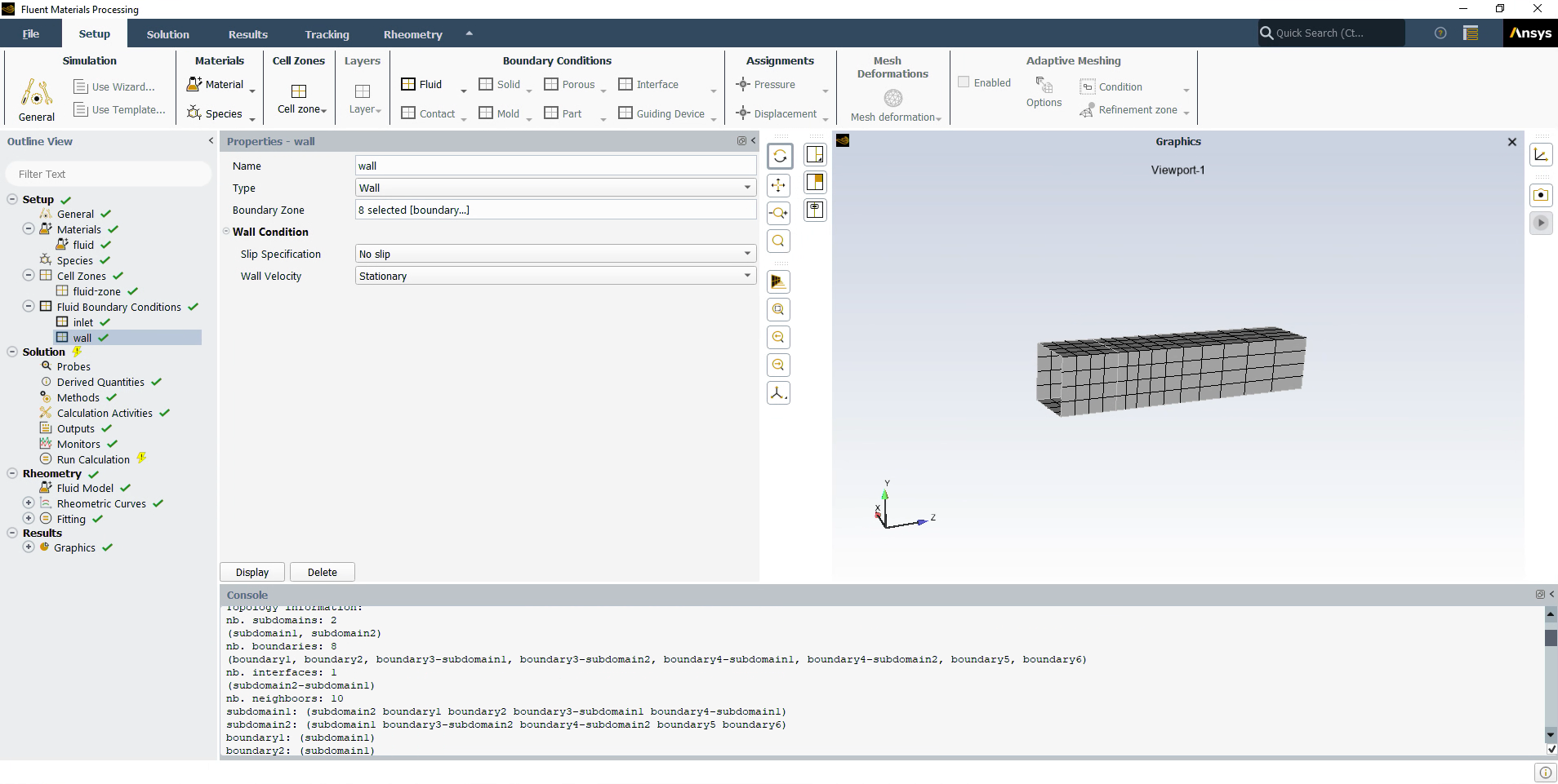
When setting up your simulation, the majority of your actions will start by performing actions in the Ribbon or the Outline View, and the associated Properties panels.
The workspace Ribbon represents a horizontal workflow, and is structured similarly to, and interacts with, elements of the Outline View. As you progress from left to right, creating or editing objects (such as create a New... or Edit... an existing object from the Fluid Boundary Condition item), elements of the ribbon become available, and objects become visible in the Outline View.
In the Ribbon, the simulation can be defined by adding objects from the Setup section of the ribbon.

Solution-specific options are accessible from the Solution section
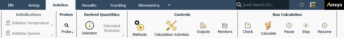
Data from a complete simulation can be analyzed by adding objects in the Results section. This includes predefined, Quick-view postprocessing objects such as Velocity, Pressure, or Temperature (if applicable) contour plots. In addition, for shell and film applications, Thickness is also available as a quick-view postprocessing object such that, if there are several layers present, you can show the total thickness of all layers, and if there is only a single layer, you can easily plot its thickness.

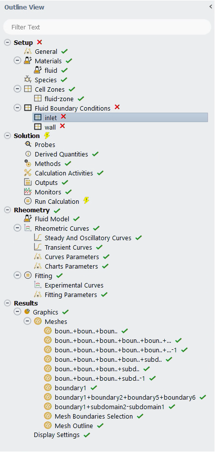
In the Outline View, the simulation can be defined by adding objects to the Setup section of the tree, solution-specific options are accessible from the Solution section, while the data from a simulation can be analyzed by adding objects in the Results section.
You can perform wildcard and regular expression searches in the tree using the
filter text entry box at the top of the tree where you can search and organize a
list using a text string. The text string can include wildcards and regular
expressions, which allow you to perform pattern matching. For example, searching
*let* finds surfaces such as
inlets and outlets, including those
with longer names, such as "upper-inlet-5". If you have walls separated by a
number, you can search example-wall-?-23, which would
show example-wall-1-23,
example-wall-2-23, and so on. Filtering begins as soon
as you enter text. Clicking Enter expands any sub-branches
containing matches to the entered string.
Icons help you visualize the status of an object in the Outline View. For
instance,  represents the state of an object whose inputs are fully defined, whereas
 represents
the state where an object still requires attention, providing you with a quick
visualization of the state of your simulation setup. In addition,
represents
the state where an object still requires attention, providing you with a quick
visualization of the state of your simulation setup. In addition,  under
Solution indicates that the solution must be
calculated.
under
Solution indicates that the solution must be
calculated.
Right-click an item in the Outline View and use the menu that opens to perform a function (such as create a New... object from the Fluid Boundary Condition item); and you can left-click an item to open a related Properties window.
The Properties windows are similar to task pages or dialog boxes, in that they allow you to define settings, run the calculation, and postprocess results. Note that your settings are saved as you define them in a Properties window, unlike dialog boxes (which you may open from the Outline View or settings in the Properties window) which require you to click an button.
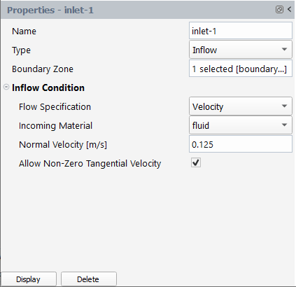
Properties that require your attention will be highlighted in red. Valid inputs will be highlighted in green.
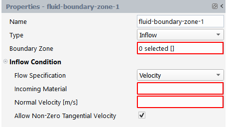
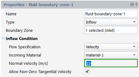
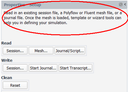
In most cases, explanatory text and/or informational messages can appear at the top of the property window in order to guide you through your workflow.
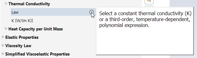
Note: Field-level user assistance (available by hovering next to a field and
clicking on the field's exposed help icon - ![]() ) is available
for many fields of the workspace, however, it is not available on Linux, or
when using ACT.
) is available
for many fields of the workspace, however, it is not available on Linux, or
when using ACT.
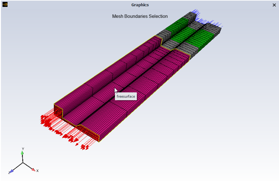
The graphics window lets you visualize the mesh that you have read into the Fluent Materials Processing workspace. Depending on the task, the graphics window will be updated to show relevant information. For example, when you are setting flow boundary conditions, the mesh outline will be shown and the selected boundary set will change color.
Use the toolbars to manipulate the model view and to change various sub-window (or viewport) settings (see Using the Toolbars). You can also use the mouse to manipulate the view of the model in the graphics window. Graphics window colors and mouse mappings can be customized to your liking using preferences (see Setting Preferences for Fluent Materials Processing).
Additional visual indicators are employed to convey even more information, if applicable, such as:
Zone highlighting and identification when hovering over and/or selecting a zone
Arrows (also known as boundary markers) indicating flow direction. For instance, red arrows indicate flow direction for outlets, blue arrows indicate flow direction for inlets, and gray arrows indicate the side of the mold body for shell geometries. In addition, blue darts on fluid cell zones for shell geometries indicate the direction of the applied inflation pressure.
Small, semi-transparent spheres indicating the location of the probes, pressure assignment, displacement assignment
Semi-transparent planes, along the boundary line (for shell geometries with symmetry planes) or at a specified point (for guiding devices such as conveyors), oriented following the specified normal
Semi-transparent boundaries, boxes, or spheres for adaptive meshing zones, depending on their type, size, and location.
The Fluent Materials Processing workspace provides a console window that displays useful information about your setup and solution, such as licensing details, your working directory, messages, and other details related to your work, in addition to access to Python scripting.
Note: The console window in the Fluent Materials Processing workspace does not provide access to a text user interface (TUI) as it does in the Fluent Solution workspace
Note: While you can enter Python commands directly in the console, ideally, you should instead read Python commands directly from a journal file, as this allows for each command to complete before the next command is executed. This is especially important for interdependent commands. Typing or pasting a series of Python commands directly into the console could result in undesirable behavior, as there is no waiting for the previous command to complete before the next command is executed.
The console window provides configurable access to warning and error messages, as described in The Console in the Fluent User's Guide for the Fluent Solution workspace.
Use the "arrange the workspace" drop-down (![]() ) in the upper-right of the workspace window to dock
(minimize) or tab the console within a separate dialog:
) in the upper-right of the workspace window to dock
(minimize) or tab the console within a separate dialog:
Dock or minimize the console by selecting the Console>Minimize option
Tab the console alongside warning and errors tabs in the Messages dialog box by selecting the Console> In Message Window option.
Access the Messages dialog box using the icon (
 ) located in the lower right hand corner of the
workspace.
) located in the lower right hand corner of the
workspace.
You can specify global settings that are applied whenever you are operating in Fluent Materials Processing. These settings are case-independent and are controlled using the Preferences dialog box.
![]() File
→ Preferences...
File
→ Preferences...
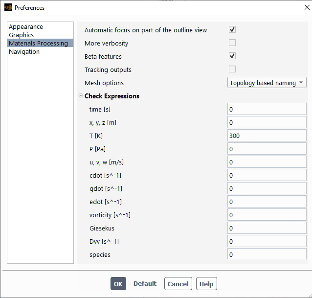
Preferences specific to the Fluent Materials Processing workspace can be found under Materials Processing.
The Automatic focus on part of the outline view option, enabled by default, automatically collapses the Outline View for the other nodes when they are not in focus. For instance, if you are navigating through the Setup node of the tree, then the Solution and Results node are automatically collapsed for easier viewing of overly-populated tree structures.
The More verbosity option lets you increase the level of detail present in messages and informational text displayed the transcripts generated by the workspace.
The Beta features option exposes features that are not yet fully supported.
The Tracking outputs option
For more information on current beta features, see Fluent Materials Processing Workspace.The Mesh options drop-down list lets you determine an optimal method for managing mesh objects. You can choose to use
Standard naming, creates and displays mesh objects in the Outline View using a standard naming convention format (for example, mesh-1, mesh-2, mesh-3, and so forth).
Topology based naming (default), creates and displays mesh objects in the Outline View using a naming convention based on the topology names found in the mesh file, with a maximum of 40 characters (for example inlet, outlet, freesurface+wall, and so forth).
User meshes only, displays only your own mesh objects in the Outline View and makes them available for use in scenes, etc. (with the exceptions the Mesh Outline and the Mesh Boundaries Selection mesh objects).
The Check Expressions group contains the available variables that can be used in expressions, and default values that can be adjusted accordingly.
Important: The following Mouse Mappings settings (under Navigation) are not supported by the Fluent Materials Processing workspace:
Select Toggle
Box Select Toggle
Probe
Box Select Add
Box Select
Set View Center
Show Menu or Probe
Note: Many of the preferences apply to the Fluent Solution workspace, and some apply to the Meshing workspace, while still others apply to their specific workspaces or workflows within Fluent. Other preferences, such as themes and generated file locations can be applied to all workspaces. For more general information about Fluent preferences, see Setting User Preferences/Options
The Fluent Materials Processing workspace includes toolbars located within the application window. These toolbars provide shortcuts to performing common tasks in the workspace.
The pointer tools allow you to modify the way in which you view your model or select objects in the graphics window. The following is a description of each of the pointer tools:
Rotate View
 lets you rotate your model about a central
point in the graphics window. For more information, see Controlling the Mouse Button Functions.
lets you rotate your model about a central
point in the graphics window. For more information, see Controlling the Mouse Button Functions.Pan
 allows you to pan horizontally or vertically
across the view using the left mouse button. For more information,
see Controlling the Mouse Button Functions.
allows you to pan horizontally or vertically
across the view using the left mouse button. For more information,
see Controlling the Mouse Button Functions.Zoom In/Out
 allows you to zoom in to and out of the model
by holding the left mouse button down and moving the mouse down or
up. For more information, see Controlling the Mouse Button Functions. You can also roll the view
by holding the left mouse button down and moving the mouse left or
right.
allows you to zoom in to and out of the model
by holding the left mouse button down and moving the mouse down or
up. For more information, see Controlling the Mouse Button Functions. You can also roll the view
by holding the left mouse button down and moving the mouse left or
right.Zoom to Area
 allows you to focus on any part of your model.
After selecting this option, position the mouse pointer at a corner
of the area to be magnified, hold down the left mouse button and
drag open a box to the desired size, and then release the mouse
button. The enclosed area will then fill the graphics window. Note
that you must drag the mouse to the right in order to zoom in. To
zoom out, you must drag the mouse to the left. For more information,
see Controlling the Mouse Button Functions.
allows you to focus on any part of your model.
After selecting this option, position the mouse pointer at a corner
of the area to be magnified, hold down the left mouse button and
drag open a box to the desired size, and then release the mouse
button. The enclosed area will then fill the graphics window. Note
that you must drag the mouse to the right in order to zoom in. To
zoom out, you must drag the mouse to the left. For more information,
see Controlling the Mouse Button Functions.
The view tools allow you to modify the way your model is displayed in the graphics window. The following is a description of each of the view tools:
 shows the 3D object on your 2D screen
approximately how your eye would see it in real life. This button is
only available when running the workspace in 3D.
shows the 3D object on your 2D screen
approximately how your eye would see it in real life. This button is
only available when running the workspace in 3D. shows 3D objects to scale, ignoring perspective
view. When enabled, it makes it so the ruler is
accurate. This button is only available when running the
workspace in 3D.
shows 3D objects to scale, ignoring perspective
view. When enabled, it makes it so the ruler is
accurate. This button is only available when running the
workspace in 3D.Fit to Window
 adjusts the overall size of your model to take
maximum advantage of the graphics window’s width and
height.
adjusts the overall size of your model to take
maximum advantage of the graphics window’s width and
height.Last View
 allows you to revert to the displayed object's
previous location and orientation in the graphics window.
allows you to revert to the displayed object's
previous location and orientation in the graphics window.Next View
 allows you to proceed to the displayed object's
next location and orientation in the graphics window, given a
collection of views provided by the use of the Last
View tool ( ).
allows you to proceed to the displayed object's
next location and orientation in the graphics window, given a
collection of views provided by the use of the Last
View tool ( ).Set view
 contains a drop-down of views, allowing you to
display the model from the direction of the vector equidistant to
all three axes, as well as in different axes orientations.
contains a drop-down of views, allowing you to
display the model from the direction of the vector equidistant to
all three axes, as well as in different axes orientations.
The graphics window in the Fluent Materials Processing workspace consists of one or more viewports where you can visualize your model and your results. A single viewport can be duplicated and each can be arranged in different layouts, presenting different views of the same model, all in a single graphics window. The following is a brief description of the available viewport arrangement tools:
Set Layout
 allows you to select from a collection of
viewport arrangements.
allows you to select from a collection of
viewport arrangements.Set Active Viewport
 allows you to select a viewport and make it
active.
allows you to select a viewport and make it
active.Link Viewports
 synchronizes the display of the selected
viewports.
synchronizes the display of the selected
viewports.
The visibility tool allow you to modify the appearance of objects in the graphics window. The following is a brief description of the available visibility tool:
Axes Visibility
 turns the axes display on and off.
The standard toolbar (Figure 4.4: The Standard Toolbar) contains options for getting help, arranging the graphical user interface, and visiting the Ansys website.

The following is a brief description of each of the standard toolbar options:
Help
 allows you to access the Fluent User's Guide for help
topics. For more information, see Using the Help System.
allows you to access the Fluent User's Guide for help
topics. For more information, see Using the Help System.Arrange the workspace
 provides you with several application window
layout options. For example, you can choose to hide certain windows
or have the graphics window be much larger than the other elements.
These options also allow you to return to a standard layout if you
accidentally rearrange (by dragging and dropping, or closing
elements) the workspace in an undesirable manner.
provides you with several application window
layout options. For example, you can choose to hide certain windows
or have the graphics window be much larger than the other elements.
These options also allow you to return to a standard layout if you
accidentally rearrange (by dragging and dropping, or closing
elements) the workspace in an undesirable manner.Link to the Ansys Website
 opens a link to the Ansys home page in
your default browser.
opens a link to the Ansys home page in
your default browser.
The following topics outline useful information about using the workspace.
As you proceed to define your simulation setup, you will often need to add objects to refine the simulation. Often, there are several ways to add objects to your simulation, whether it is using the Outline View, the Ribbon, or the Properties panel.
For instance, to create a new condition for adaptive meshing, you can use either of the following approaches:
Using the Properties panel, at the bottom of the Adaptive Meshing properties, select the Add a Condition button.
 Setup → Adaptive
Meshing
Setup → Adaptive
Meshing Using the Outline View, with the context menu:
Setup → Adaptive
Meshing  Add a
condition
Add a
condition or without the context menu:
Setup → Adaptive
Meshing
→ Conditions → condition-1
Using the Ribbon:
 Setup → Adaptive
Meshing → Condition
→ New
Setup → Adaptive
Meshing → Condition
→ New
Of course, with the ability to add objects, you can also remove objects from your simulation using the corresponding Delete option/button.
Fluent expressions are available when using the Fluent Materials Processing workspace. As described in Fluent Expressions Language, Fluent expressions are an interpreted, declarative language based on Python, enabling you to specify complex boundary conditions and/or model settings.
Note: Units should not be included in any expressions used in the Fluent Materials Processing workspace.
Note: When using time as a variable in an expression,
the variable must be called "time" (in lower
case) and cannot be abbreviated (say to use "t"
instead).
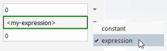
You can customize the behavior of a quantity or property using expressions. If you are able to apply an expression to a quantity or property in the workspace, a drop-down menu provides you the choice of selecting a constant value or an expression. If you select expression, then you are able to enter an expression using the Fluent expression language.
For transient simulations, expressions are allowed for the following scenarios, and for the following quantities:
Table 4.1: Expression-Supported Quantities for Transient Simulations
| Condition | Category | Quantity | Available for Transient? | Available for Continuation? | Available for Volume of Fluid? |
|---|---|---|---|---|---|
|
Solid cell zone |
Transport Velocity |
Vx | yes | ||
|
Vy | yes | ||||
|
Vz | yes | ||||
|
Mold cell zone |
Translation Velocity |
Vx | yes | ||
|
Vy | yes | ||||
|
Vz | yes | ||||
|
General Motion |
Omega | yes | |||
|
Vx | yes | ||||
|
Vy | yes | ||||
|
Vz | yes | ||||
| Fluid cell zone | Volume Conservation |
Initial Fluid Volume | yes | ||
| Inflation Pressure |
Time Dependency | yes | |||
| Normal Flow Rate Condition |
Volume Flow Rate | yes | yes | ||
|
General |
Gravity Vector |
Gx | yes | yes | |
|
Gy | yes | yes | |||
|
Gz | yes | yes | |||
|
Inflow |
Volume Flow Rate | yes | yes | yes | |
|
Mass Flow Rate | yes | yes | yes | ||
|
Normal Velocity | yes | yes | yes | ||
| Outflow |
Volume Flow Rate | yes | yes | yes | |
|
Mass Flow Rate | yes | yes | yes | ||
|
Normal Velocity | yes | yes | yes | ||
|
Pressure | yes | yes | yes | ||
|
Wall (partial slip) |
Navier Law |
Friction Coefficient | yes | yes | yes |
|
Generalized Navier Law |
Friction Coefficient | yes | yes | yes | |
|
Threshold Law |
First Friction Coefficient | yes | yes | yes | |
|
Second Friction Coefficient | yes | yes | yes | ||
|
Generalized Threshold Law |
First Friction Coefficient | yes | yes | yes | |
|
Second Friction Coefficient | yes | yes | yes | ||
|
Asymptotic Law |
Friction Coefficient | yes | yes | yes | |
|
Temperature Dependence |
Ea/R | yes | yes | yes | |
|
Extrudate exit | Take-up Force per Unit Area | yes | yes | ||
|
Take-up Velocity |
Vx | yes | yes | ||
|
Vy | yes | yes | |||
|
Vz | yes | yes | |||
|
Take-up Force |
Fx | yes | yes | ||
|
Fy | yes | yes | |||
|
Fz | yes | yes | |||
|
Porous Wall |
Temperature Dependence |
Ea/R | yes | yes | yes |
|
Thermal (for fluid, solid, and porous boundary conditions) |
Temperature | yes | yes | yes | |
|
Heat Flux | yes | yes | yes | ||
|
Heat Transfer Coefficient | yes | yes | yes | ||
|
Convection Temperature | yes | yes | yes | ||
| Fluid/Solid Interface |
Navier Law |
Friction Coefficient | yes | yes | yes |
|
Generalized Navier Law |
Friction Coefficient | yes | yes | yes | |
|
Threshold Law |
First Friction Coefficient | yes | yes | yes | |
|
Second Friction Coefficient | yes | yes | yes | ||
|
Generalized Threshold Law |
First Friction Coefficient | yes | yes | yes | |
|
Second Friction Coefficient | yes | yes | yes | ||
|
Asymptotic Law |
Friction Coefficient | yes | yes | yes | |
|
Temperature Dependence |
Ea/R | yes | yes | yes |
Table 4.2: Expression-Supported Properties for Transient Simulations (Materials)
| Property | Category | Quantity | Available for Transient? | Available for Continuation? | Available for Volume of Fluid? | |
|---|---|---|---|---|---|---|
| Viscosity Law | Shear Dependency | Power law | Power Law Index | yes | yes | yes |
| Bird-Carreau Law | Power Law Index | yes | yes | yes | ||
| Carreau-Yasuda Law | Power Law Index | yes | yes | yes | ||
| Bingham Law | Critical Shear Rate | yes | yes | yes | ||
| Modified Bingham Law | Critical Shear Rate | yes | yes | yes | ||
| Herschel-Bulkley Law | Power Law Index | yes | yes | yes | ||
| Critical Shear Rate | yes | yes | yes | |||
| Modified Herschel-Bulkley Law | Power Law Index | yes | yes | yes | ||
| Critical Shear Rate | yes | yes | yes | |||
| Cross law | Cross Law Index | yes | yes | yes | ||
| Modified Cross Law | Cross Law Index | yes | yes | yes | ||
| Temperature dependence | Arrhenius | Ea/R | yes | yes | yes | |
| Approximate Arrhenius | Ea/R | yes | yes | yes | ||
| Fulcher | F2 | yes | yes | yes | ||
| WLF | C1 | yes | yes | yes | ||
| Simplified Viscoelastic Properties | Weighting Coefficient | yes | yes | yes | ||
| Shear Rate Dependency | Power law | Power Law Index | yes | yes | yes | |
| Bird-Carreau Law | Power Law Index | yes | yes | yes | ||
| Carreau-Yasuda Law | Power Law Index | yes | yes | yes | ||
| Cross law | Cross Law Index | yes | yes | yes | ||
| Modified Cross Law | Cross Law Index | yes | yes | yes | ||
| First Normal Viscosity | Power law | Power Law Index | yes | yes | yes | |
| Bird-Carreau Law | Power Law Index | yes | yes | yes | ||
| Carreau-Yasuda Law | Power Law Index | yes | yes | yes | ||
| Cross law | Cross Law Index | yes | yes | yes | ||
| Modified Cross Law | Cross Law Index | yes | yes | yes | ||
| Relaxation Time Law | Power law | Expor | yes | yes | yes | |
| Bird-Carreau Law | Expor | yes | yes | yes | ||
| Thermal Dependence | Arrhenius | Ea/R | yes | yes | yes | |
| Approximate Arrhenius | Ea/R | yes | yes | yes | ||
| WLF | C1 | yes | yes | yes | ||
| Thermal Properties | Thermal conductivity | A / K | yes | yes | yes | |
| Heat Capacity | A / Cp | yes | yes | yes | ||
| Viscosity Law in Porous Medium | Temperature Dependence | Arrhenius | Ea/R | yes | yes | yes |
| Approximate Arrhenius | Ea/R | yes | yes | yes | ||
| Integral Viscoelastic Properties | Temperature Dependence | Arrhenius | Ea/R | yes | ||
| Approximate Arrhenius | Ea/R | yes | ||||
| WLF | C1 | yes | ||||
| Differential Viscoelastic Properties | Temperature Dependence | Arrhenius | Ea/R | yes | yes | yes |
| Approximate Arrhenius | Ea/R | yes | yes | yes | ||
| WLF | C1 | yes | yes | yes | ||
Often material properties are nonlinear algebraic functions of the
primary field variables, such as temperature, pressure, and chemical
species, to name a few. The Fluent Materials Processing workspace allows you to customize
the definition of material properties by defining one or more functions.
This can be done by defining a Fluent expression on such properties
(for example, the heat capacity can be written as Cp = 200 +
x * (T-300) * 10.
Generalized expressions can be functions of the following variables:


Note: Variable names used in expressions should not be used as species nicknames.
Note: Default values for these expression variables are provided in the Preferences dialog box, (see Setting Preferences for Fluent Materials Processing) and can be adjusted accordingly.
Generalized expressions (applicable to steady, transient, continuation and VOF simulations) can be defined for the following properties:
Table 4.3: Generalized Expression-Supported Properties (General)
| Category | Quantity | Available for Steady? | Available for Transient? | Available for Continuation? | Available for Volume of Fluid? |
|---|---|---|---|---|---|
| Gravity | Gx | yes | yes | yes | yes |
| Gy | yes | yes | yes | yes | |
| Gz | yes | yes | yes | yes |
Table 4.4: Generalized Expression-Supported Properties (Materials)
| Property | Category | Quantity | Available for Steady? | Available for Transient? | Available for Continuation? | Available for Volume of Fluid? |
|---|---|---|---|---|---|---|
| Viscosity Law | Constant Law | Viscosity | yes | yes | yes | yes |
| Density Law | Density | yes | yes | yes | yes | |
| Simplified Viscoelastic Properties | Viscosity Law / Constant Law | Viscosity | yes | yes | yes | yes |
| Thermal Properties | Thermal Conductivity | A / K | yes | yes | yes | yes |
| Heat Capacity | A / Cp | yes | yes | yes | yes |
Table 4.5: Generalized Expression-Supported Properties (Cell Zones)
| Category | Quantity | Available for Steady? | Available for Transient? | Available for Continuation? | Available for Volume of Fluid? |
|---|---|---|---|---|---|
| 2D Film / 2D Shell | Heat Transfer Coefficient | yes | yes | yes | yes |
| Convective Temperature | yes | yes | yes | yes | |
| Other Geometry Types | Heat Source per Unit Volume | yes | yes | yes | yes |
Table 4.6: Generalized Expression-Supported Properties (Boundary Conditions - Thermal)
| Category | Quantity | Available for Steady? | Available for Transient? | Available for Continuation? | Available for Volume of Fluid? |
|---|---|---|---|---|---|
| Fluid, Solid, Porous, Mold | Heat Transfer Coefficient | yes | yes | yes | yes |
| Convective Temperature | yes | yes | yes | yes |
Table 4.7: Generalized Expression-Supported Properties (Boundary Conditions - Species)
| Category | Quantity | Available for Steady? | Available for Transient? | Available for Continuation? | Available for Volume of Fluid? |
|---|---|---|---|---|---|
| Fluid | Transfer Coefficient | yes | yes | yes | yes |
| Reference Species | yes | yes | yes | yes |
Table 4.8: Generalized Expression-Supported Properties (Species)
| Category | Quantity | Available for Steady? | Available for Transient? | Available for Continuation? | Available for Volume of Fluid? |
|---|---|---|---|---|---|
| Transport | Source term | yes | yes | yes | yes |
| Scalar diffusivity | yes | yes | yes | yes |
Note: You should not define an expression on density for a solid, a porous medium, (fluid and solid fractions), or a mold. If present, the workspace will detect such an expression while checking the simulation setup.
An expression can be applied to density to model a compressible flow. For such flows with variable overall density, one has to solve the mass conservation equation. The overall density is either treated as an additional variable or algebraically substituted. The treatment used depends on the nature of the term to be evaluated: if a gradient must be computed, then the density is considered as a variable; if an algebraic relationship must be computed, then the density is simply substituted. The resulting formulation is a mixed method with an increase in the number of unknown variables. This solution procedure, however, has several advantages. The implementation is rather easy and, most importantly, it allows you to model an equation of state of any kind while still keeping the Newton-Raphson rate of convergence. When the density varies, velocity is no longer divergence-free, as it is for incompressible flows. Since mass is conserved, the flow kinematics as well as the volume of the material may change dramatically. For example, consider a problem in which the density decreases as chemical reactions proceed. In a confined geometry, the fluid will accelerate; in a free surface problem, large swelling ratios will be observed, and it may be useful to consider a gradual solution strategy using a continuation technique to introduce this nonlinearity
Note: If you define an expression for density, you must also define:
an average density in the density law, to be used for initializing the calculations,
the density at the inlet(s) of the flow simulation.
If the fluid cell zone includes multiple materials, then the cell zone cannot be combined with foaming and/or transport of species and/or generalized expressions defined on material properties.
If the fluid cell zone includes foaming, then the cell zone cannot be combined with multiple materials and/or transport of species and/or generalized expressions defined on material properties.
If an expression is defined on density, you cannot impose a mass flow rate at the inlets and/or the outlets.
While expressions can be written and tested in the Fluent Expressions Editor, the editor's inclusion of units can be an issue when used in the Fluent Materials Processing workspace. Most expressions employ a syntax similar to Excel such that an expression can be written and tested in Excel to ensure proper syntax. This section discusses some common types of expressions that you can easily re-use in your simulation.
Note: Function names included in expressions must be lower case.
The following list contains a collection of expressions that can be useful when working in the Fluent Materials Processing workspace.
Linear function of time
Description:
function = value * time
Example:
0.001 * time
Function of inverse of time
Description:
function = value / time
Note: Time cannot be equivalent to 0.
Example:
0.001 / time
Polynomial function of time
Description:
function = value * ( a + b*time + c*time^2 + d*time^3 + e*time^4 )
Example:
0.001 * (0.1+0.2*time+0.3*time^2+0.4*time^3+0.5*time^4)
Ramp function of time
Description:
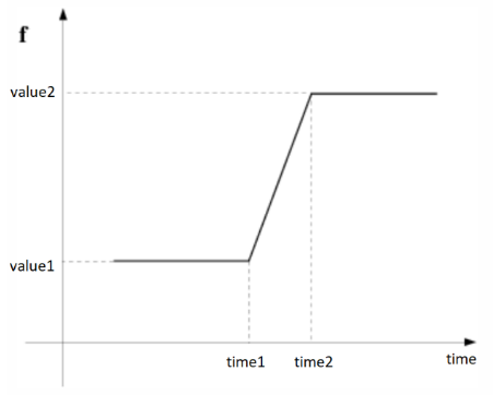
function = IF(time <= time1,value1,
                    IF(time>=time2,value2,
                        value1+(value2-value1)/(time2-time1)*(time-time1)
                    )
           )
Example:
IF(time <= 0.8, 0.1,
        IF(time >= 0.9, 0.2, 0.1+(0.2-0.1)/(0.9-0.8)*(time-0.8)
        )
)
Cosine function of time
Description:
function = value * ( a + cos(b*time + c) + d + e*time )
Example:
0.001 *(0.1*cos(0.2*time+0.3)+0.4+0.5*time)
Power function of time
Description:
function = value * ( a *time^b + c*time^d )
Example:
0.001 *(0.1*time^0.2+0.3*time^0.4)
Exponential function of time
Description:
function = value * ( a *exp(b*time) + c + d*time )
Example:
0.001 *(0.1*exp(0.2*time)+0.3+0.4*time)
Double ramp function of time
Description:
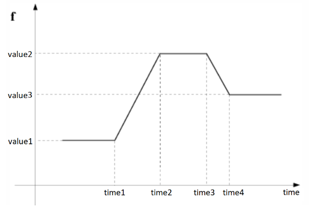
function = IF(time <= time1,value1,
             IF(time<=time2,value2, value1+(value2-value1)/(time2-time1)*(time-time1)
               IF(time<=time3,value2,
                 IF(time>=time4,value3, value2+(value3-value2)/(time4-time3)*(time-time3)
                 (
               )
              )
            )
Example:
IF(time <= 1.1, 0.1,
         IF(time <= 1.2,0.1+(0.2-0.1)/(1.2-1.1)*(time-1.1),
           IF(time<=1.3,0.2,
             IF(time>=1.4,0.3,
                0.2+(0.3-0.2)/(1.4-1.3)*(time-1.3)))))
Piecewise function of time
Description:
function = IF(time <= time1,value1,
            IF(time<=time2, value1+(value2-value1)/(time2-time1)*(time-time1)
                IF(time<=time3, value2+(value3-value2)/(time3-time2)*(time-time2),
                    IF(time<=time4, value3+(value4-value3)/(time4-time3)*(time-time3),value4)
                )
             )
           )
Example:
IF(time <= 1.1, 0.1,
        IF(time <= 1.2,0.1+(0.2-0.1)/(1.2-1.1)*(time-1.1),
         IF(time<=1.3,0.2+(0.3-0.2)/(1.3-1.2)*(time-1.2),
          IF(time<=1.4,0.3+(0.4-0.3)/(1.4-1.3)*(time-1.3),0.4))))
Heaviside unit function of time
Description:
function = IF(time < time1,0,1)
Example:
IF(time < 1.1, 0.,1.)
Range function of time
Description:
function = IF(time <= time1,0,
            IF(time>=time2,0,1))
Example:
IF(time <= 1.1,0.,IF(time >= 1.2,0.,1.))
Gaussian function of time
Description:
function = a * exp(-((time-b)/c)^2)
Example:
0.1*exp(-((time-0.2)/0.3)^2)
Power function of 2 fields
Description:
function = a * X1^b * X2^c
Example:
0.1*X1^0.2*X2^0.3
Polynomial function of 2 fields
Description:
function = X1*(a+b*X2+c*X2^2+d*X2^3)
Example:
X1*(0.1+0.2*X2+0.3*X2^2+0.4*X2^3)
Exponential function of inverse
Description:
function = a*exp ( b / (X1 + c) )
Example:
0.1*exp(-200./ (X1-0.2))
Natural logarithm
Description:
function = a*log ( b * (X1 + c) )
Example:
0.1*log(0.2*(X1*0.3))
Decimal logarithm
Description:
function = a*log10 ( b * (X1 + c) )
Example:
0.1*log10(0.2*(X1*0.3))
Use the help menu (![]() ) icon in the upper right-hand corner of the workspace to
access its documentation. Some workspaces even have field-level user assistance
that provide information and guidance about a particular field.
) icon in the upper right-hand corner of the workspace to
access its documentation. Some workspaces even have field-level user assistance
that provide information and guidance about a particular field.
In addition to Online Technical Resources..., and the Product Improvement Program, you can also obtain information about the version and release of Fluent you are running by selecting the Version... option in help menu.