This chapter include several Material Processing Examples for Ansys Fluent.
The information in this chapter is divided into the following sections:
- 4.1. Spinning Simulation of a Non-Symmetric Trilobal Viscoelastic Fiber
- 4.2. Reinforcements and Pantographing in Rubber Tire Molding
- 4.3. 3D Non-isothermal Flow with a Non-conformal Mesh
- 4.4. Extrusion of a Foamed Profile
- 4.5. Filling of a Sample
- 4.6. 3D Structure Interaction for Die
- 4.7. Thermal Simulation of the Internal Flow of a Fluid in a Channel with One Entry and Four Exits
- 4.8. Multilayer Film Casting
- 4.9. Extrusion of a Rubber Profile With a Metal Insert
- 4.10. Extrusion of a D-Fender
This example is divided into the following sections:
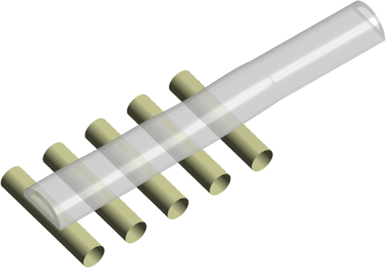
In the process of synthetic fiber spinning, a filament of polymer is stretched, usually at high speed, in order to achieve a fiber with a very small cross-section area. For fibers with a circular cross-section, the die shape is not an issue. Other fibers may have a more complex shape, presumably for the optical properties that can be produced. The tri-lobal fiber has again a well-known level of symmetry. For the purpose of generality, a fiber cross-section that has no symmetry is considered.
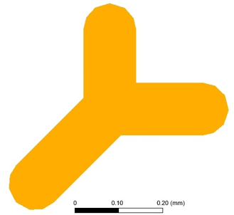
Figure 4.1: Non-symmetric Die Cross-section for a Tri-lobal Fiber, displays the cross section of the die used for the production of the tri-lobal fiber. In the present case, the length of all three lobes, measured from the center to the tip, are of 0.24, 0.27 and 0.30 mm, respectively for the vertical, the horizontal and the sloped lobe. The lobes width is 0.12 mm, while the curvature radius is 0.06 mm. In addition, the angular distribution of the lobes further enhances the (purposely selected) non-symmetric geometric shape.
This example is designed to illustrate the setup of a viscoelastic flow, and at the same time, to show the effects of viscoelasticity on the fiber shape. For describing the rheology of the melt, the Oldroyd-B model is purposely selected, which is known to exhibit a strong transient elongation viscosity. In a single mode context, the model involves three parameters: the relaxation time, the zero-shear viscosity, and the viscosity of a purely Newtonian component (solvent). For the relaxation time, the value 0.02 s is chosen. The value may appear low, but it is of a similar order of magnitude as the residence time of a fluid particle in the calculation domain. By doing so, a visible development of viscoelastic effects is allowed. For both viscosity factors, the values 80 and 20 Pa.s are selected, respectively.
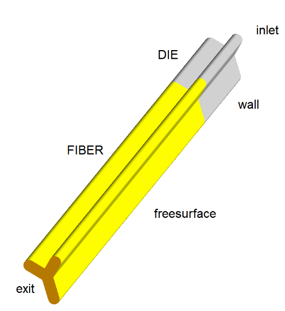
The three-dimensional calculation domain is shown in Figure 4.2: Non-symmetric Tri-lobal Fiber Spinning: Calculation Domain and Boundaries, along with the named selections for all of the boundaries. Note that zone and boundary names are intuitive, and this helps for setting up the case. Other names are certainly possible, preferably as long as you can unambiguously identify the several entities, for limiting the risk of mistakes. A flow rate Q is imposed at the inlet, slip conditions are applied on the die wall, free surface conditions are imposed on the free jet, while a take-up force is imposed at the outlet. It is also important to keep in mind that the geometric shape of the jet is a priori unknown. In the initial configuration, the cross section of the extruded fiber coincides with that of the die, while the jet would be straight.
With SI units, the following numerical values are selected for the various data involved. A flow rate of 10-8 m3/s is imposed at the inlet while a take-up force of -10-3 N is applied at the exit of the computational domain. Eventually, slipping obeying Navier's law is assumed along the die wall, where the coefficient is set to 107 Pa.s/m
The following sections describe the setup and solution steps for this example:
To prepare for running this example:
Download the
Trilobal_VE.zipfile here .Unzip
Trilobal_VE.zipto your working directory.The file,
Trilobal_VE.poly, can be found in the folder.Use Fluent Launcher to start the Fluent Materials Processing workspace, with the Capability Level set to Enterprise.
For this example, choose a simulation template for extrusion. When using a template, the Fluent Materials Processing workspace creates a skeleton based on your choice, so that usually you only need to fill in the few fields. Typically, fluid material data need to be provided. Cell zones must be defined, boundary conditions must be assigned, mesh deformation algorithm (for the fiber part) must be specified, and the calculation of derived quantities must be activated as appropriate. Eventually, solver options have to be selected before running the calculation.
![]() Setup → Simulation → Use
Template...
Setup → Simulation → Use
Template...
This displays the Simulation Template dialog box, where you can specify particular details for the type of simulation.
Set the Type to Extrusion.
Set the Goal to Predict extrudate shape.
Click Apply to close the dialog box. The workspace will set up the various requirements for the specified simulation type.
Define the differential viscoelastic material properties for the fluid.
![]() Setup → Materials →
fluid
Setup → Materials →
fluid
Expand the Differential Viscoelastic Properties in the properties view.
Set the Model to Oldroyd-B.
Set the Number of Relaxation Modes to 1.
Set the Additional Viscosity to 20 Pa s.
Set the Relaxation Time to 0.02 s.
Set the Partial Viscosity to 80 Pa s.
Define the cell zone properties for the fluid-zone.
![]() Setup → Cell Zones →
fluid-zone
Setup → Cell Zones →
fluid-zone
Set the Zones to include die and fiber.
Set the Fluid Model to Differential viscoelastic.
Set the Fluid Material(s) to fluid.
Define the conditions for the various boundaries in the simulation.
Define conditions at the extrudate-exit.
 Setup → Fluid Boundary
Conditions → extrudate-exit
Setup → Fluid Boundary
Conditions → extrudate-exitSet the Boundary Zone to exit.
Set the Flow Specification to Take-up force.
Set the Take-up Force components Fx, Fy, and Fz to 0 N, 0 N, and -0.001 N, respectively.
Define conditions at the free-surface.
Setup → Fluid Boundary
Conditions → free-surfaceSet the Boundary Zone to freesurface.
Set the Fixed Part to wall (the attachment line of the free surface).
Define conditions at the inlet.
Setup → Fluid Boundary
Conditions → inletSet the Boundary Zone to inlet.
Set the Flow Specification to Volume flow.
Set the Incoming Material to fluid.
Set the Volume Flow Rate to 1e-8 m3/s.
Define conditions at the wall.
Setup → Fluid Boundary
Conditions → wallSet the Boundary Zone to wall.
Set the Slip Specification to Partial slip.
Set the Slip Model to Navier law.
Set the Friction Coefficient to 1e7 kg/m2s.
Define the conditions for the various mesh deformations in the simulation, that is, the extrudate.
![]() Setup → Mesh Deformations
→ extrudate
Setup → Mesh Deformations
→ extrudate
Set the Zones to fiber.
Set the Extrudate Deformation Method to Streamwise.
Set the Inlet Section to fiber-die.
Set the Outlet Section to exit.
Define any particular solution-based settings in the simulation.
Define any derived quantities.
Solution → Derived Quantities Select Stress if you want to have access to the total extra-stress tensor for subsequent examination.
Select any other quantities that are of interest.
Define any calculation activities.
Solution → Calculation
Activities Set the Number of Processors to 4.
For Convergence Strategies, select Free Surfaces and Moving Interfaces and Viscoelasticity.
Run the calculations.
The setup is now ready and it can now be checked, and the calculation can start.
Solution → Run Calculation Click Check to perform a final check of the setup and the coherence of the data.
If there are no errors or warnings, click Calculate.
With the current mesh, the calculation requires approximately one hour, and eight continuation steps until completion.
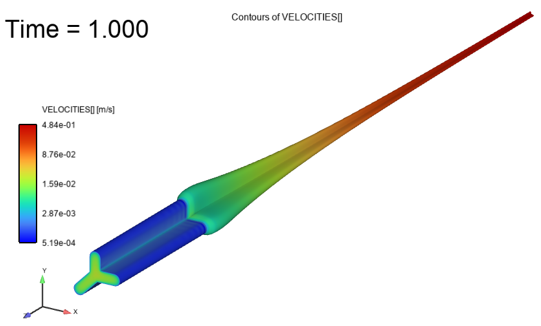
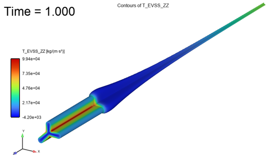
In this example, it is assumed that you are already familiar the graphical analysis tools of the workspace. Figure 4.3: Spinning of a Tri-lobal Viscoelastic Fiber - Velocity Distribution displays contours of the velocity magnitude with a log scale together with the fiber shape. You can see that the velocity on the die wall is very low, resulting from the selected friction coefficient. Under the application of a take-up force of -10‑3 N, a fiber velocity of about 0.48 m/s is obtained at the end of the computational domain. Under the application of the same force, an inelastic material with identical viscosity would exhibit a velocity of about 1.8 m/s at the end of the computational domain. This visible reduction of the take-up velocity results from the fast-growing transient elongational viscosity of the Oldroyd-B model.
A further inspection of the results reveals that the local shear rate reaches values up to approximately 165 s‑1 along the die wall. In the fiber itself, the largest value is of about 100 s‑1. Here it has to be understood as an image of the actual (and local) strain rate. An examination of the stress tensor component along the z-axis (main flow direction) also reveals that large values are encountered. When the relaxation time decreases, therefore when strain hardening decreases, a smaller fiber cross-section is observed, and this can be accompanied by larger elongation (normal) stress in the fiber. Figure 4.4: Spinning of a Tri-lobal Viscoelastic Fiber - Distribution of the Axial Extra-stress Component displays the distribution of the axial component of the extra-stress tensor on the entire boundary of the computational domain. In the present context, this component is a fingerprint of the first normal stress difference along the die wall, and of the take-up stress in the fiber at some distance from the die exit.
Figure 4.4: Spinning of a Tri-lobal Viscoelastic Fiber - Distribution of the Axial Extra-stress Component
This example is divided into the following sections:
This example demonstrates a simple simulation for the shaping of a rubber tire. A relatively simple geometric model is considered for the rubber assembly and for the mold. The assembly consists of four layers: the reinforced carcass, the sidewalls, the reinforcement belts, and the tread. For all four layers, a simple rheological model is considered for the rubber matrix. The carcass is reinforced with fabric cords while the reinforcement belts are merged into a single belt reinforced with two sets of wires. For modeling the fabric cords and wires, an orthotropic fluid model is used.
The concept of reinforced or orthotropic fluid model consists of an isotropic fluid matrix, which is reinforced by means of one or several systems of cords or wires. This reinforcement structure confers a specific orthotropic viscosity to the matrix: since the deformation is hindered along the direction of orthotropy. When deformations of the fluid system are significant, it may be necessary to update the orientation of the reinforcement system accordingly.
For the present purpose, tread patterns are omitted, and a simple mold geometry is proposed to enable a relatively fast simulation for a complex industrial application. In Figure 4.5: Problem Description: The Open Mold (a) and the Initial Assembly (b), both mold parts and the assembly are displayed in their respective initial configurations.. A cross section is made in the assembly for easily identifying the four layers considered. It is here assumed that the assembly is completed before being placed into the mold.
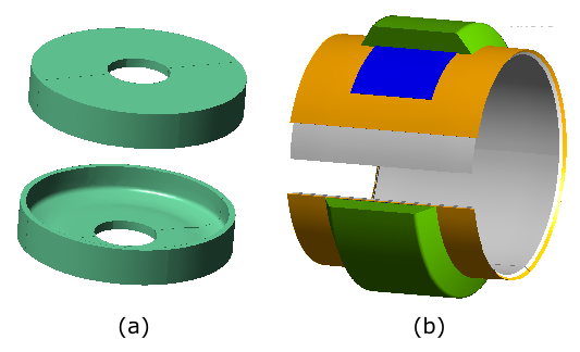
The mold and assembly are displayed with different scales. The four layers presently considered are the carcass (grey), the sidewalls (orange), the reinforcement belts (blue) and the tread (green).
In terms of reinforcements, fabric cords are embedded into the carcass along the axial direction. Two sets of wires are considered in the reinforcement belts with a well-defined initial relative angle. During shaping, the distribution of relative angle will change along with the deformation of the assembly. This mechanism is often referred to as pantographing.
In the present application, the outer diameter of the tire, the height and the width are of 736, 155 and 218 mm, respectively. Following the ETRTO norm (European Tyre and Rim Technical Organization) used in the rubber tire industry, the present tire model would be assigned the classification number 215/70R17.
For computational reasons, only a quarter of the geometry shown in Figure 4.5: Problem Description: The Open Mold (a) and the Initial Assembly (b) is considered and is displayed in Figure 4.6: Problem Description - One Quarter Geometry.
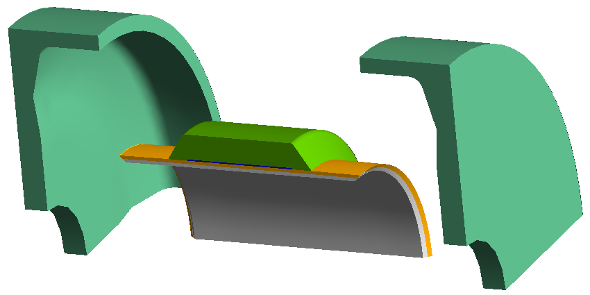
A quarter of the geometry displays the open mold and the assembly, both mold and assembly are displayed with the same scale.
For all four layers considered here, the same rubber matrix is selected. Since the primary focus is the prediction of pantographing that occurs during tire molding, a simple Newtonian model is purposely selected for describing the fluid behavior. The rubber is characterized by a constant (Newtonian) viscosity of 105 Pa.s and a density of 1200 kg/m3.
The fabric cords in the carcass are initially oriented along the axis of the cylinder, and a reinforcement magnitude of 107 Pa.s is considered. The sets of cords in the reinforcement belts have an initial orientation of +40° and ‑40° with respect to the traveling direction, respectively. A reinforcement magnitude of 107 Pa.s is also considered.
The process starts by shaping a pre-tire: this is performed by applying an axial motion to both extremities of the assembly via an appropriate time-dependent velocity boundary condition. For this, velocities of ‑0.028 and +0.028 m/s are assigned respectively at the top and at the bottom ring, and which linearly decreases to 0 within the time interval [2.95, 3.05].
Upon completion of this phase, the pre-tire is virtually inserted into the mold, which is then closed. Both molds are initially at a distance of 0.4 m with each other. Mold motion is imposed within the time interval [3.5, 4.05], with velocities of ‑0.4 and +0.4 m/s assigned respectively to the upper and lower mold within the time interval [3.55, 4.0] and with a linear variation from and to 0, respectively within the intervals [3.5, 3.55] and [4.0, 4.05]. For the contact treatment, default values of 1012 are kept for the penalty and slipping coefficients while the penetration accuracy is set to 10‑3 m.
Together with these velocity conditions, a slight pre-blowing pressure is applied on the inner surface of the assembly to prevent possible buckling. Subsequently the blowing pressure is applied in order to shape the tire. More precisely, a pre-blowing pressure of 20,000 Pa is applied until time t=2.5 s. During the time interval [2.6, 4.7], there is zero pressure and eventually, the shaping pressure increases from 0 up to 7 105 Pa within the time interval [4.7, 5.8], and keeps this value afterwards.
From the modeling point of view, four sub-domains are defined for the layers of the assembly, and two additional domains are created for the molds. Interface conditions are defined between successive layers of the assembly. Free surface boundary conditions with a time-dependent inflation pressure are considered for the inner surface of the assembly, while free surface conditions with contact are considered for the outer surface. At both extremities of the assembly, half of the area is treated as a free surface, while a time-dependent velocity is imposed on the other half.
The initial calculation domain for the assembly is discretized by means of 16000 elements (all layers considered). Both molds are discretized by means of about 6000 elements each. Since relatively large deformations are expected, adaptive meshing will be invoked after each sequence of 5 steps, this is set by default. A minimum element size of 0.01 m is selected.
With the concept of reinforced fluid model or orthotropic fluid model, the following can be understood. A matrix of isotropic fluid is considered, that is reinforced along a given direction by means of rigid rods, fibers, fabric cords or wires. From this, it is quite natural to consider a constitutive model, which consists of a part for the unreinforced matrix and a part for the reinforcement structure. Hence, within the context of a fluid model, the reinforcement structure is described by means of the direction of orthotropy and a reinforcement magnitude along this direction. The reinforcement magnitude has the units of a viscosity and can be, for example, 100 times the zero-shear viscosity of the matrix. The reinforcement structure confers a specific orthotropic viscosity to the system. With one set of oriented reinforcement rods, deformation is hindered along the selected direction, while the matrix can still deform along the other directions. With two sets of reinforcement rods, the global behavior will be more intricate.
For an object whose initial configuration is flat, specifying the initial orientation of the reinforcement cords or wires is relatively straightforward. This is also the case for a cylindrical object when the reinforcement cords or wires are initially oriented along its axis. For cylindrical objects involving helix-like reinforcement cords or wires, the orientation will be defined with respect to a plane perpendicular to the axis of the cylinder.
Simulation of pressing case necessarily involves the prediction of contact that occurs between the processed material and a mold. Next to a mesh supporting the fluid domain, a mesh must also be defined for the mold. In isothermal situations, the mesh is needed for the geometry only, and the discretization can be coarse. When a heat exchange between fluid and mold is calculated, care must also be taken for the discretization of the mold.
A Lagrangian representation is used for performing the simulation of pressing cases. In other words, finite elements will deform on the same way as the fluid, and at regular interval, a new finite element mesh has to be recreated. This is the purpose of adaptive meshing: it is activated by default with a set of parameters that you can adjust accordingly.
Based on the original problem description, you can see that five input data are a function of time. There is the axial velocity imposed at both extremities of the assembly, the velocity applied on both molds, and the shaping pressure. This section reviews these time-dependences.
The process starts by shaping a pre-tire: this is performed by applying an axial motion to
both extremities of the assembly via an appropriate time-dependent velocity boundary condition.
For this, ramp expressions are defined on the y-component of the velocity, which vary from
‑0.028 and +0.028 m/s respectively at the top and at the bottom ring to 0 within the
time interval [2.95, 3.05]. The corresponding expressions for the upper and lower extremities
of the assembly are respectively given by expression-1:
IF(time <= 2.95, -0.028,
    IF(time >= 3.05, 0.,
        -0.028+(0.+0.028)/(3.05-2.95)*(time-2.95)
      )
  )
and expression-2:
IF(time <= 2.95, 0.028,
    IF(time >= 3.05, 0.,
        0.028+(0.-0.028)/(3.05-2.95)*(time-2.95)
      )
  )
Time dependent functions are also used for describing the motion assigned to the molds.
Both molds are initially at a distance of 0.4 m with each other. Here, double-ramp expressions
are defined on the y-velocity component of the molds: velocities vanish before time=3.5 s and
beyond time=4.05 s, they are set to ‑0.4 and +0.4 m/s respectively to the upper and
lower mold within the time interval [3.55, 4.0] s, while they linearly vary from 0 and to 0
within the remaining time intervals [3.5, 3.55] and [4.0, 4.05] s, respectively. The
corresponding expressions for the upper and lower molds are respectively given by
expression-3:
IF( time <= 3.5, 0.,
    IF( time <= 3.55, 0.+(-0.4-0.)/(3.55-3.5)*(time-3.5),
        IF( time <= 4., -0.4,
            IF( time <= 4.05, -0.4+(0.+0.4)/(4.05-4.)*(time-4.),
                0.
              )
          )
      )
  )
and expression-4:
IF( time <= 3.5, 0.,
    IF( time <= 3.55, 0.+(0.4-0.)/(3.55-3.5)*(time-3.5),
        IF( time <= 4., 0.4,
            IF( time <= 4.05, 0.4+(0.-0.4)/(4.05-4.)*(time-4.),
                0.
              )
          )
      )
  )
Eventually, a slight pre-blowing pressure is applied on the inner surface of the assembly
to prevent possible buckling, and the blowing pressure is subsequently applied in order to
shape the tire. More precisely, a pre-blowing pressure of 20,000 Pa is applied until time t=2.5
s where it then decreases down to 0 at time=2.6 s. At time=4.7 s, it increases again until
time=5.8 s where it reaches a value of 7 105 Pa, which is then
maintained. The corresponding expression for the pressure is given by the
expression-5:
IF( time <= 2.5, 0.2e5,
    IF( time <= 2.6, 0.2e5+(0.-0.2e5)/(2.6-2.5)*(time-2.5),
        IF( time <= 4.7, 0.,
            IF( time <= 5.8, 0.+(7.e5-0.)/(5.8-4.7)*(time-4.7),
                7.e5
              )
          )
      )
  )
The following sections describe the setup and solution steps for this example:
- 4.2.2.1. Preparation
- 4.2.2.2. Mesh
- 4.2.2.3. Simulation Settings
- 4.2.2.4. Materials
- 4.2.2.5. Cell Zones
- 4.2.2.6. Fluid Boundary Conditions
- 4.2.2.7. Interface Boundary Conditions
- 4.2.2.8. Contact Boundary Conditions
- 4.2.2.9. Mesh Deformations
- 4.2.2.10. Adaptive Meshing
- 4.2.2.11. Solution Settings
- 4.2.2.12. Postprocessing
To prepare for running this example:
Download the
Tire_Manufacturing.zipfile here .Unzip
Tire_Manufacturing.zipto your working directory.The file,
tire_manufacturing.polycan be found in the folder.Use Fluent Launcher to start the Fluent Materials Processing workspace, with the Capability Level set to Enterprise.
For this example, choose a simulation template for pressing. When using a template, the Fluent Materials Processing workspace creates a skeleton based on your choice, so that usually you only need to fill in the few fields. In view of the complexity of the present pressing case, you will have to create several new fields and fill them accordingly. Typically, fluid material data need to be provided. Cell zones must be defined for the layers of the assembly as well as for the molds, including the motion of the molds, boundary, interface and contact conditions must be assigned, mesh deformation algorithm and adaptive meshing (for the assembly) must be specified, and the calculation of derived quantities must be activated as appropriate. Eventually, solver options must be selected before running the calculation.
![]() Setup → Simulation → Use
Template...
Setup → Simulation → Use
Template...
This displays the Simulation Template dialog box, where you can specify particular details for the type of simulation.
Set the Type to Pressing.
Set the Number of Moving Molds to 2.
Set the Duration to 6 seconds.
Click Apply to close the dialog box. The workspace will set up the various requirements for the specified simulation type.
In particular, entries are created for the cell zones (including both molds), the fluid boundary conditions and contact conditions, as well as for the mesh deformations and the adaptive meshing.
Here, you will define the materials for the simulation.
Define the material properties for the existing fluid (fluid).
Setup → Materials →
fluid Set the Name to carcass.
Expand the Density Law and set the Density to 1200 kg/m3.
Expand the Viscosity Law and set the Viscosity to 100000 (or 1e5) Pa s.
Expand the Reinforcement Properties and set the Number of Reinforcements to 1.
For the 1-st Reinforcement, set the following properties:
Set the Magnitude to 1e7 Pa s.
Set the X-component of Reinforcement to 0.
Set the Y-component of Reinforcement to 1.
Create a new material for the sidewall.
Setup → Materials
 New...
 Set the Name to sidewall.
Expand the Density Law and set the Density to 1200 kg/m3.
Expand the Viscosity Law and set the Viscosity to 100000 (or 1e5) Pa s.
Create a new material for the belts.
Setup → Materials
New... Set the Name to belts.
Expand the Density Law and set the Density to 1200 kg/m3.
Expand the Viscosity Law and set the Viscosity to 100000 (or 1e5) Pa s.
Expand the Reinforcement Properties and set the Number of Reinforcements to 2.
For the 1-st Reinforcement, set the following properties:
Set the Magnitude to 1e7 Pa s.
Set the Orientation to Cylindrical domain.
Set the Cylinder Axis to Y-axis.
Set the Angle of Reinforcement to 40.
For the 2-nd Reinforcement, set the following properties:
Set the Magnitude to 1e7 Pa s.
Set the Orientation to Cylindrical domain.
Set the Cylinder Axis to Y-axis.
Set the Angle of Reinforcement to -40.
Create a new material for the tread.
Setup → Materials
New... Set the Name to tread.
Expand the Density Law and set the Density to 1200 kg/m3.
Expand the Viscosity Law and set the Viscosity to 100000 (or 1e5) Pa s.
Here, you will define specific cell zones in the simulation.
Define the cell zone properties for the existing fluid cell zone (fluid-zone).
Setup → Cell Zones →
fluid-zone Change the Name to Carcass.
Set the Zones to carcass.
Set the Fluid Material(s) to carcass.
Expand the Volume Conservation and deactivate it.
Expand the Matrix Reinforcement and activate it.
Define the cell zone properties for the first moving mold (moving-mold-1).
Setup → Cell Zones →
moving-mold-1 Change the Name to Mold-down.
Set the Zones to molddown.
Expand Mold Motion and Translation Velocity and for Vy, and select expression from the drop-down list.
Enter the contents of
expression-4.IF( time <= 3.5, 0., IF( time <= 3.55, 0.+(0.4-0.)/(3.55-3.5)*(time-3.5), IF( time <= 4., 0.4, IF( time <= 4.05, 0.4+(0.-0.4)/(4.05-4.)*(time-4.), 0. ) ) ) )
Define the cell zone properties for the second moving mold (moving-mold-2).
Setup → Cell Zones →
moving-mold-2 Change the Name to Mold-up.
Set the Zones to moldup.
Expand Mold Motion and Translation Velocity and for Vy, and select expression from the drop-down list.
Enter the contents of
expression-3.IF( time <= 3.5, 0., IF( time <= 3.55, 0.+(-0.4-0.)/(3.55-3.5)*(time-3.5), IF( time <= 4., -0.4, IF( time <= 4.05, -0.4+(0.+0.4)/(4.05-4.)*(time-4.), 0. ) ) ) )
Define a new cell zone for the sidewall and set its properties.
Setup → Cell Zones
New... Change the Name to Sidewall.
Set the Zones to sidewall.
Set the Fluid Material(s) to sidewall.
Expand the Volume Conservation and deactivate it.
Define a new cell zone for the belts and set its properties.
Setup → Cell Zones
New... Change the Name to Belts.
Set the Zones to belts.
Set the Fluid Material(s) to belts.
Expand the Volume Conservation and deactivate it.
Expand the Matrix Reinforcement and activate it.
Define a new cell zone for the tread and set its properties.
Setup → Cell Zones
New... Change the Name to Tread.
Set the Zones to tread.
Set the Fluid Material(s) to tread.
Expand the Volume Conservation and deactivate it.
Define the conditions for the various fluid boundaries in the simulation.
Define conditions at the free-surface.
Setup → Fluid Boundary
Conditions → free-surfaceChange the Name to Inner.
Set the Boundary Zone to inner.
Expand Free Surface Conditions, and for Gauge Pressure, select expression from the drop-down list.
Enter the contents of
expression-5.IF( time <= 2.5, 0.2e5, IF( time <= 2.6, 0.2e5+(0.-0.2e5)/(2.6-2.5)*(time-2.5), IF( time <= 4.7, 0., IF( time <= 5.8, 0.+(7.e5-0.)/(5.8-4.7)*(time-4.7), 7.e5 ) ) ) )
Define a new fluid boundary condition for the bottom free surface and set its properties.
Setup → Fluid Boundary
Conditions New... Change the Name to FSbot.
Set the Type to Free surface.
Set the Boundary Zone to ringbot-carcass.
Define a new fluid boundary condition for the top free surface and set its properties.
Setup → Fluid Boundary
Conditions New... Change the Name to FStop.
Set the Type to Free surface.
Set the Boundary Zone to ringtop-carcass.
Define a new fluid boundary condition for the outer sidewall free surface and set its properties.
Setup → Fluid Boundary
Conditions New... Change the Name to FSsidewall.
Set the Type to Free surface.
Set the Boundary Zone to outer-sidewall.
Define a new fluid boundary condition for the outer tread free surface and set its properties.
Setup → Fluid Boundary
Conditions New... Change the Name to FStread.
Set the Type to Free surface.
Set the Boundary Zone to outer-tread.
Define a new fluid boundary condition for yz symmetry plane and set its properties.
Setup → Fluid Boundary
Conditions New... Change the Name to Symm-x.
Set the Type to Symmetry.
Set the Boundary Zone to symmx-belts, symmx-carcass, symmx-sidewall, and symmx-tread.
Define a new fluid boundary condition for xy symmetry plane and set its properties.
Setup → Fluid Boundary
Conditions New... Change the Name to Symm-z.
Set the Type to Symmetry.
Set the Boundary Zone to symmz-belts, symmz-carcass, symmz-sidewall, and symmz-tread.
Define a new fluid boundary condition for the bottom ring of the sidewall and set its properties.
Setup → Fluid Boundary
Conditions New... Change the Name to Ringbot.
Set the Type to Wall.
Set the Boundary Zone to ringbot-sidewall.
Under Wall Condition, set the Wall Velocity to Moving.
Under First Point of Axis, set the X1, Y1, and Z1 to (0,0,0) respectively.
Under Second Point of Axis, set the X2, Y2, and Z2 to (0,1,0) respectively.
Set the Angular Velocity to 0.
Under Translation Velocity:
Set Vx to 0.
For Vy, select expression from the drop-down list, and enter the contents of
expression-2:IF(time <= 2.95, 0.028, IF(time >= 3.05, 0., 0.028+(0.-0.028)/(3.05-2.95)*(time-2.95) ) )Set Vz to 0.
Define a new fluid boundary condition for the top ring of the sidewall and set its properties.
Setup → Fluid Boundary
Conditions New... Change the Name to Ringtop.
Set the Type to Wall.
Set the Boundary Zone to ringtop-sidewall.
Under Wall Condition, set the Wall Velocity to Moving.
Under First Point of Axis, set the X1, Y1, and Z1 to (0,0,0) respectively.
Under Second Point of Axis, set the X2, Y2, and Z2 to (0,1,0) respectively.
Set the Angular Velocity to 0.
Under Translation Velocity:
Set Vx to 0.
For Vy, select expression from the drop-down list, and enter the contents of
expression-1:IF(time <= 2.95, -0.028, IF(time >= 3.05, 0., -0.028+(0.+0.028)/(3.05-2.95)*(time-2.95) ) )Set Vz to 0.
Here, you will define the conditions at the interface boundaries.
Create a new interface boundary condition between the sidewall and the carcass.
Setup → Interface Boundary
Conditions New... Set the Name to Int_carcass_sidewall.
Set the Type to Fluid-Fluid.
Set the Interface Zone to sidewall-carcass.
Create a new interface boundary condition between the sidewall and the belts.
Setup → Interface Boundary
Conditions New... Set the Name to Int_sidewall_belts.
Set the Type to Fluid-Fluid.
Set the Interface Zone to belts-sidewall.
Create a new interface boundary condition between the sidewall and the tread.
Setup → Interface Boundary
Conditions New... Set the Name to Int_sidewall_tread.
Set the Type to Fluid-Fluid.
Set the Interface Zone to tread-sidewall.
Create a new interface boundary condition between the belts and the tread.
Setup → Interface Boundary
Conditions New... Set the Name to Int_belts_tread.
Set the Type to Fluid-Fluid.
Set the Interface Zone to belts-tread.
Here, you will define various contact boundary conditions for the simulation.
Define contact boundary conditions at the first moving mold contact-with-moving-mold-1.
Setup → Contact Boundary
Conditions → contact-with-moving-mold-1Change the Name to Sidewall_up.
Set the Fluid to Sidewall.
Set the Fluid Zone of Contact to outer-sidewall.
Set the Mold to Mold-up.
For the Mold Zone of Contact, select cup.
Set the Penetration Accuracy to 0.001 m.
Define contact boundary conditions at the second moving mold contact-with-moving-mold-2.
Setup → Contact Boundary
Conditions → contact-with-moving-mold-2Change the Name to Tread_up.
Set the Fluid to Tread.
Set the Fluid Zone of Contact to outer-tread.
Set the Mold to Mold-up.
For the Mold Zone of Contact, select cup.
Set the Penetration Accuracy to 0.001 m.
Create a new contact boundary condition for the outer sidewall and the mold.
Setup → Contact Boundary
Conditions New... Set the Name to Sidewall_down.
For the Fluid, select Sidewall.
For the Fluid Zone of Contact, select outer-sidewall.
For the Mold, select Mold-down.
For the Mold Zone of Contact, select cbottom.
Set the Penetration Accuracy to 0.001 m.
Create a new contact boundary condition for the outer tread and the mold.
Setup → Contact Boundary
Conditions New... Set the Name to Tread_down.
For the Fluid, select Tread.
For the Fluid Zone of Contact, select outer-tread.
For the Mold, select Mold-down.
For the Mold Zone of Contact, select cbottom.
Set the Penetration Accuracy to 0.001 m.
Define the conditions for the various mesh deformations in the simulation.
Define conditions at the existing fluid deformation (fluid-deformation).
Setup → Mesh Deformations
→ fluid-deformationChange the Name to Carcass.
Set the Zones to carcass.
Create a new mesh deformation for the sidewall.
Setup → Mesh Deformations
New... Set the Name to Sidewall.
For the Type, select Lagrangian.
For the Zones, select sidewall.
Create a new mesh deformation for the belts.
Setup → Mesh Deformations
New... Set the Name to Belts.
For the Type, select Lagrangian.
For the Zones, select belts.
Create a new mesh deformation for the tread.
Setup → Mesh Deformations
New... Set the Name to Tread.
For the Type, select Lagrangian.
For the Zones, select tread.
Here, you will set various adaptive meshing criteria.
![]() Setup → Adaptive Meshing
Setup → Adaptive Meshing
Under the main properties for Adaptive Meshing, disable the Mapping feature.
Edit the existing adaptive meshing condition (condition-1).
Change the Name to condition-carcass.
For the Zones, select carcass.
Under Condition on Mesh Quality, set the Size to 0.01 m.
Disable the Condition on Contact by clearing the Enabled check box.
Create a new adaptive meshing condition for the sidewall.
Setup → Adaptive Meshing
→ Conditions New... Set the Name to condition-sidewall.
For the Zones, select sidewall.
Enable the Condition on Mesh Quality by checking the Enabled check box, and set the Size to 0.01 m.
Create a new adaptive meshing condition for the belts.
Setup → Adaptive Meshing
→ Conditions New... Set the Name to condition-belts.
For the Zones, select belts.
Enable the Condition on Mesh Quality by checking the Enabled check box, and set the Size to 0.01 m.
Create a new adaptive meshing condition for the tread.
Setup → Adaptive Meshing
→ Conditions New... Set the Name to condition-tread.
For the Zones, select tread.
Enable the Condition on Mesh Quality by checking the Enabled check box, and set the Size to 0.01 m.
Define any particular solution-based settings in the simulation.
Define specific solution methods.
Solution → MethodsUnder Contact Parameters, set the Element Dilitation to User value, and set the User Dilitation to 1e-5 m.
Define any calculation activities.
Solution → Calculation
Activities Set the Number of Processors to 5.
Run the calculations.
The setup is now ready and it can now be checked, and the calculation can start.
Solution → Run Calculation Click Check to perform a final check of the setup and the coherence of the data.
If there are no errors or warnings, click Calculate.
With the current mesh, the calculation requires approximately one hour, and about 130 time steps are needed until completion.
Figure 4.7: Progression of the Assembly Shape,displays a sequence of snapshots of the assembly at several instants during shaping of the toroidal pre-tire until final shaping in the mold achieved at time t=6 s. Carcass, sidewall and tread are displayed in grey, orange and green, respectively. The reinforcement belts are not visible since they are located under the tread.
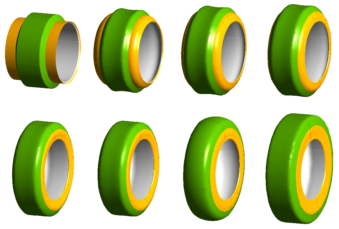
The shape of the assembly at various time steps during the simulation from the cylindrical assembly to the final tire (the mold is not displayed). The four layers presently considered are the carcass (grey), the sidewalls (orange), the reinforcement belts (blue – not displayed) and the tread (green).
Figure 4.8: Cross Section of the Final Tire Assembly displays a cross section in the final tire, where you also see the location and the final shape of the reinforcement belts shown in blue.
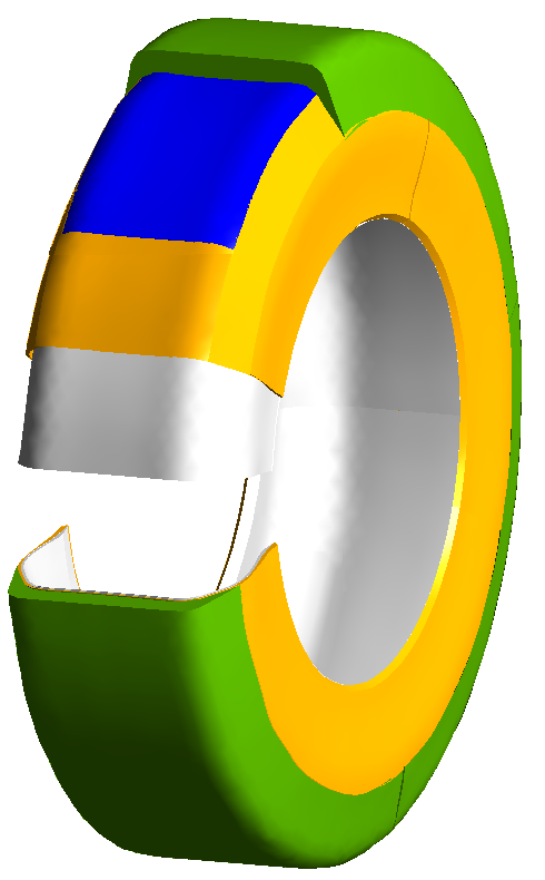
The assembly tire shape at the end of the molding phase with a cross-section through the several layers. The four layers shown are the carcass (grey), the sidewalls (orange), the reinforcement belts (blue) and the tread (green).
Figure 4.9: Inspecting the Carcass and Belts displays the configuration of the fabric cords and of the reinforcement cords on a quarter of the tire upon molding completion. Figure 4.9: Inspecting the Carcass and Belts (a) shows a few cords in the carcass and in the reinforcement belts. The lines suggesting the cords have been created as surface streamlines obtained by integrating the anisotropy vector. It is important here to understand that these lines are not actual cords. A macroscopic model is used for predicting the orientations of cords, and these lines are only a sampling out of a continuum. Figure 4.9: Inspecting the Carcass and Belts (b) displays the relative angle between both sets of cords embedded in the reinforcement belts. It is obtained from the scalar product between two vectors a and b:
 | (4–1) |
In the initial configuration of the assembly, the reinforcement cords embedded in the belts have a relative angle of 80°. Upon completion of molding, the relative angle exhibits a distribution ranging between 46° and 62°. A non-uniform pantographing has occurred, which originates from the deformation undergone by the belts. In particular, the diameter increase naturally leads to a reduction of the angle between the sets of cords. The slightly rugged aspect of the distribution of relative angle displayed in Figure 4.9: Inspecting the Carcass and Belts (b) is a consequence of the moderate discretization that was selected for the purpose of limiting the calculation time.
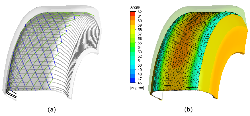
Fabric cords in the carcass and reinforcement cords in the belts (a). Relative angle between both sets of reinforcement cords in the belts (b). For clarity, the carcass (grey) and sidewalls (orange) are shown as well as the tread (transparent green).
This example is divided into the following sections:
This example illustrates a non-isothermal flow of a Newtonian liquid using a non-conformal mesh technique. This technique allows you to create a connected simulation domain out of geometrically coincident but disconnected parts. This approach facilitates the meshing of the geometry as different parts can be meshed independently.
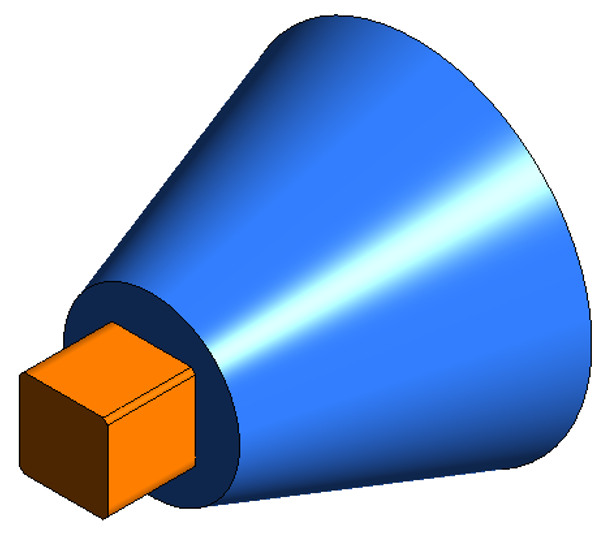
The geometry representing the three-dimensional calculation domain is depicted in Figure 4.10: Sub-domains for the 3D Non-conformal Mesh and consists of two disconnected sub-domains: the predie (in blue) and the die (in orange).
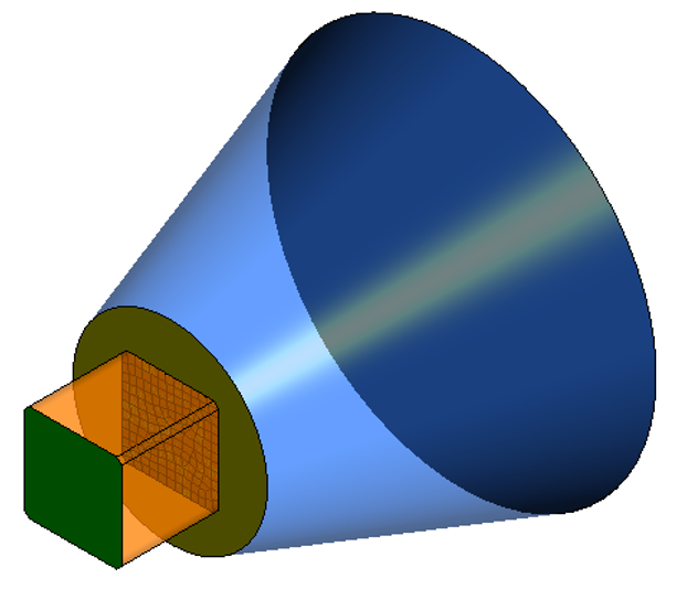
The different named selections and boundaries are shown in Figure 4.11: Boundaries for the 3D Non-conformal Mesh. The inlet is dark blue, the wall is light blue, the predieexit is yellow, the wall2 boundary is light orange, the dieexit in green, and the mesh is visible on dieentry Note that zone and boundary names are intuitive, and this helps for setting up the case.
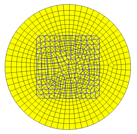
Figure 4.12: Non-conformal Mesh on the Exit of the Predie and on the Entry of the Die displays the mesh on the exit of the predie (in yellow) and on the entry of the die (in thick blue), clearly demonstrating a non-conformal nature.
A flow rate Q is imposed at the inlet, no slip conditions are applied on the predie and die walls, an outlet is defined on the die outlet.
With SI units, the following numerical values are selected for the various data involved. A flow rate of 3 10-6 m3/s is imposed at the inlet. A temperature of 373.15 K is imposed at the inlet and along the wall of the predie. A heat flux by convection is imposed along the wall of the die with a transfer coefficient of 50 W/m^2 K and a convection temperature of 353.15 K. A vanishing velocity is imposed along the walls of the predie and the die. The temperature is initialized to 373.15 K on the whole calculation domain.
The following sections describe the setup and solution steps for this example:
To prepare for running this example:
Download the
nonconformal3D.zipfile here .Unzip
nonconformal3D.zipto your working directory.The file,
nonconformal3D.poly, can be found in the folder.Use Fluent Launcher to start the Fluent Materials Processing workspace, with the Capability Level set to Enterprise.
For this example, choose a simulation template for internal flow. When using a template, the Fluent Materials Processing workspace creates a skeleton based on your choice, so that usually you only need to fill in the few fields. Typically, fluid material data need to be provided. Cell zones must be defined, boundary conditions must be assigned, and the calculation of derived quantities must be activated as appropriate. Eventually, solver options have to be selected before running the calculation.
![]() Setup → Simulation → Use
Template...
Setup → Simulation → Use
Template...
This displays the Simulation Template dialog box, where you can specify particular details for the type of simulation.
Set the Type to Internal Flow.
Enable the Thermal option.
Click Apply to close the dialog box. The workspace will set up the various requirements for the specified simulation type.
Define the material properties for the fluid.
![]() Setup → Materials →
fluid
Setup → Materials →
fluid
Expand the Density Law in the properties view.
Set the Density to 1000 kg/m3.
Expand the Thermal Properties in the properties view.
Set the Thermal Conductivity coefficient K to 0.75 W/(m K).
Set the Heat Capacity per Unit Mass coefficient Cp to 2.5 J/(kg K).
Expand the Viscosity Law in the properties view.
Set the Viscosity constant value to 200 Pa s.
Define the cell zone properties for the fluid-zone.
![]() Setup → Cell Zones →
fluid-zone
Setup → Cell Zones →
fluid-zone
Set the Zones to include predie.
Define the cell zone properties for a new fluid cell zone fluid-zone-1 (added using the Ribbon).
![]() Setup → Cell Zones →
Cell zone → New → Fluid
zone
Setup → Cell Zones →
Cell zone → New → Fluid
zone
Set the Zones to include die.
Set the Fluid Material(s) to fluid.
Define the conditions for the various boundaries in the simulation.
Define conditions at the inlet.
Setup → Fluid Boundary
Conditions → inletSet the Boundary Zone to inlet.
Set the Flow Specification to Volume flow.
Set the Volume flow rate to 3e-6 m3/s.
Set the Temperature to 373.15 K.
Define conditions at the outlet.
Setup → Fluid Boundary
Conditions → outletSet the Boundary Zone to outlet.
Define conditions at the wall.
Setup → Fluid Boundary
Conditions → wallSet the Boundary Zone to wall.
Set the Thermal Condition to Temperature.
Set the Temperature to 373.15 K.
Add a new fluid boundary condition wall-1 (using the Ribbon).
 Setup → Boundary Conditions
→ Fluid → New →
Wall
Setup → Boundary Conditions
→ Fluid → New →
WallSet the Boundary Zone to wall2.
Set the Thermal Condition to Heat flux and convection.
Set the Heat Transfer Coefficient to 50 W/(m2 K).
Set the Convection Temperature to 353.15 K.
Add a new interface fluid-fluid-1 (using the Ribbon).
Setup → Boundary
Conditions → Interface →
New → Fluid-Fluid (non-conformal)Set the Cell Zone 1 to fluid-zone.
Set the Boundary Zone 1 to predieexit.
Set the Cell Zone 2 to fluid-zone-1.
Set the Boundary Zone 2 to dieentry.
Define any particular solution-based settings in the simulation.
Define the initial temperature.
Solution → Temperature
Initializations → temperature-in-fluid-zone Set the Cell Zones to fluid-zone.
Set the coefficient A to 373.15 K.
Add a new initial temperature initial-temperature-1 (using the Ribbon).
Solution →
Initializations → Initialize
Temperature → New Keep the name as initial-temperature-1
Set the Cell Zones to fluid-zone-1.
Set the coefficient A to 373.15 K.
Define any derived quantities.
Solution → Derived Quantities Review the pre-selected derived quantities.
Select any other quantities that are of interest.
Check the solution methods.
Solution → Methods Make sure that the Upwinding in Energy Equation option is enabled.
Define any calculation activities.
Solution → Calculation
Activities Set the Number of Processors to 4.
For Convergence Strategies, keep the default settings.
Run the calculations.
The setup is now ready and it can now be checked, and the calculation can start.
Solution → Run Calculation Click Check to perform a final check of the setup and the coherence of the data.
If there are no errors or warnings, click Calculate.
In this example, it is assumed that you are already familiar the graphical analysis tools of the workspace.
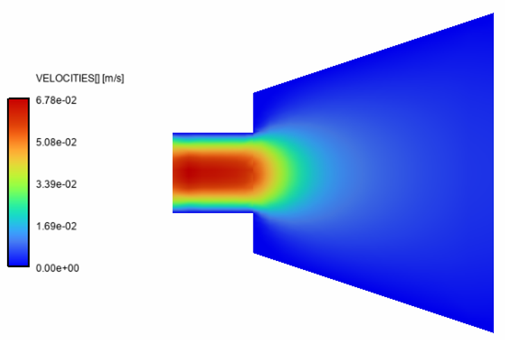
Figure 4.13: Velocity Contours in the X=0 Plane displays contours of the velocity magnitude in the center of the die
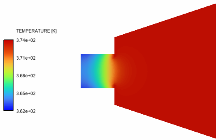
Figure 4.14: Temperature Contours in the X=0 Plane shows temperature contours on the same cutting plane. It can be observed that the velocity and the temperature are continuous through the non-conformal interface.
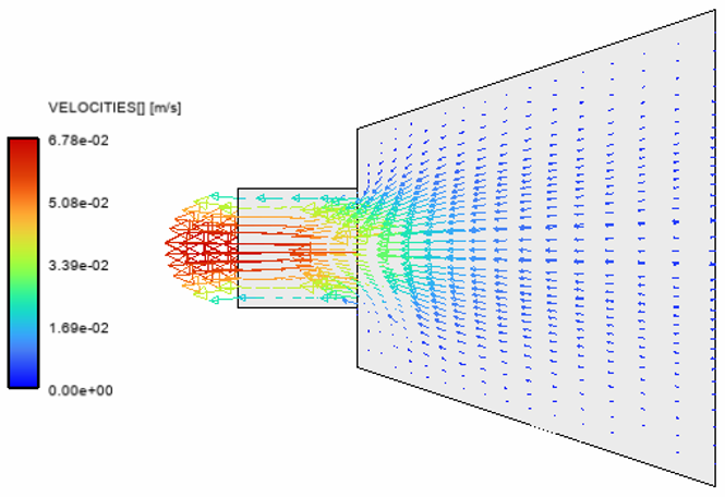
Figure 4.15: Velocity Vectors in the X=0 Plane displays velocity vectors. Again, note that the non-conforming mesh has no visible impact on the velocity field.
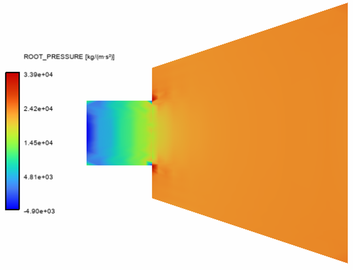
Figure 4.16: ROOT_PRESSURE Contours in the X=0 Plane displays the pressure. As there are two defined fluid zones, there are two PRESSURE fields, one for the predie and a second for the die. The ROOT_PRESSURE field is an assembly of these two fields. A pressure overshoot along the border of the actual predie exit is an expected result, as well as the small pressure undershoot along the edge of the die entry.
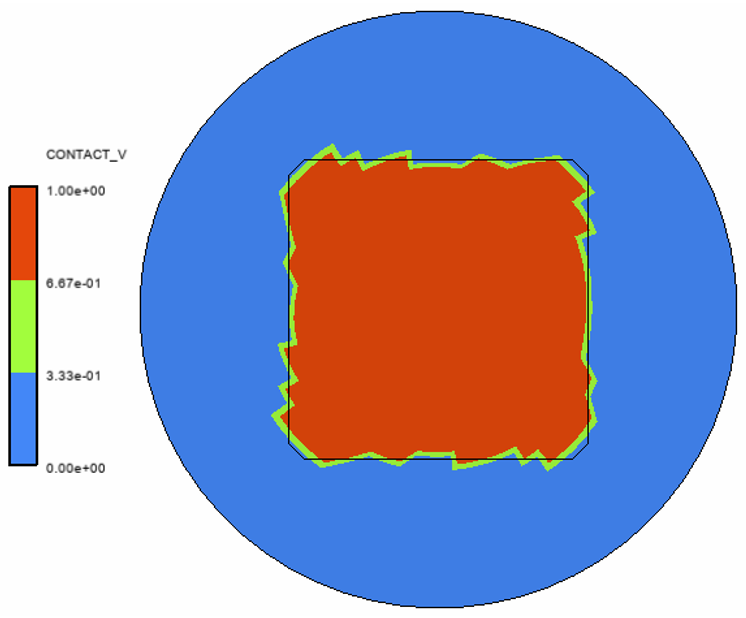
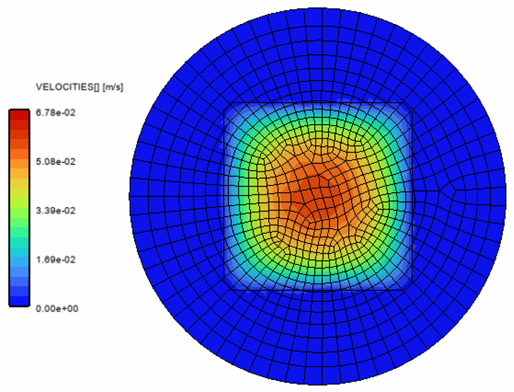
Eventually, Figure 4.17: CONTACT_V Contours on the predieexit Boundary shows that the portion of the predie exit that is overlapped by the die entry, whose border is visible in black, is actually seen in contact. The nodes not belonging to that portion of the boundary receive a vanishing velocity condition as can be seen in Figure 4.18: Velocity Contours on the predieexit Boundary
This example is divided into the following sections:
Foamed polyethylene is extruded to obtain very light insulation parts. Polyethylene with dissolved gas enters through the inlet section and flows through the converging section and the die land. Next, throughout the extrudate, the material is free to deform. The physical foaming process occurs as soon as the mixture leaves the die or at least when the pressure is low enough for allowing the gas bubbles to grow and the dissolved gas to migrate towards the microscopic bubbles.
The Arefmanesh model ([1]) is used for predicting the bubble growth. The model assumes a purely viscous material, and that the time scale of gas diffusion is longer than that of bubble expansion. The model is such that all physics is lumped in a single transport equation that dictates the bubble radius R:
 | (4–2) |
where pg is the gas pressure and
p is the matrix pressure. The parameter  may play the role of surface tension and hence prevent a possibly infinite
bubble growth. The quantity
may play the role of surface tension and hence prevent a possibly infinite
bubble growth. The quantity  is a macroscopic viscosity of the foam. The power index a
may add some non-linearities to the model but is set to 1 in this example. Eventually, parameter
b is a booster if the foaming is not as large as expected: it is also set to
1 in this example.
is a macroscopic viscosity of the foam. The power index a
may add some non-linearities to the model but is set to 1 in this example. Eventually, parameter
b is a booster if the foaming is not as large as expected: it is also set to
1 in this example.
On the other hand, the density ρ of the mixture is given by:
 | (4–3) |
where ρp is the density of the polymer matrix (without blowing agent, that is, with R equivalent to 0), and N is the number of cells per unit volume of gas/polymer mixture. Also, while foaming progresses, the macroscopic viscosity of our mixture decreases since the volume increase results only from gas expansion. Hence, with the bubble growth, the workspace assumes that the zero-shear viscosity of the mixture decreases in the same way as the density:
 | (4–4) |
where  is the zero-shear viscosity of the polymer matrix (without blowing agent, that
is, with R equivalent to 0).
is the zero-shear viscosity of the polymer matrix (without blowing agent, that
is, with R equivalent to 0).
The model does not necessarily predict an equilibrium bubble size: gas pressure decreases with increasing bubble radius but does not vanish. In actual cases, however, bubbles do not grow infinitely, since only a finite supply of gas is available for their growth, and bubbles attain equilibrium once the gas gets depleted in the polymer. Also, surface tension may eventually dominate over the remaining gas pressure.
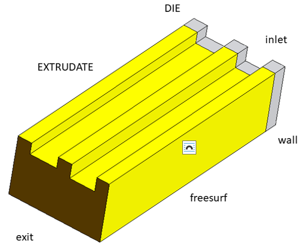
In this example, this model is to be used for the determination of die lips shape used for the extrusion of foamed profiles. For this, a 3D profile is considered and is displayed in Figure 4.19: Required Extrudate Profile . The objective is to calculate the die shape lips which will enable the extrusion of the required profile. The primary ingredient of the present example is physical foaming. In such an extrusion flow process, gas is dissolved in the polymer matrix, and will start to expand as soon as the polymer leaves the die, or at least as soon as the pressure in the polymer is low enough for the gas bubbles to expand. In order to achieve this, die lands are usually very short.
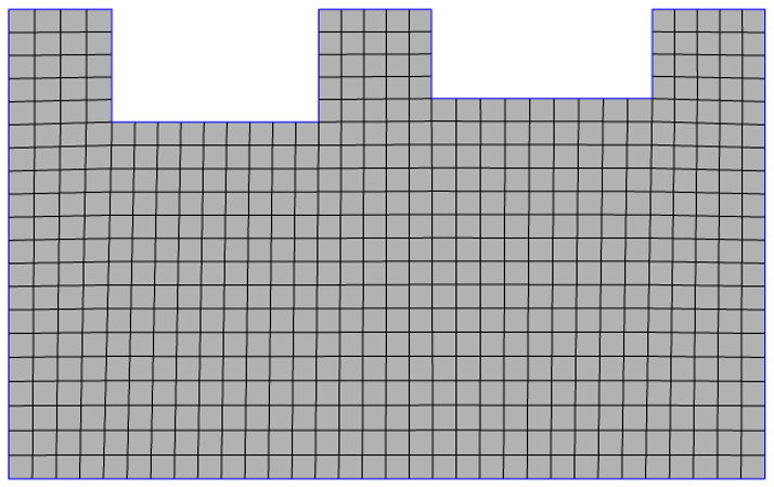
Figure 4.20: Calculation Domain and Boundaries illustrates the initial computational domain. It consists of two subdomains, a short subdomain for the die land and a long subdomain for the extrudate. Four boundaries are considered: the inlet, the die wall, the extrudate surface and the exit of the calculation domain. The corresponding boundary conditions are a volumetric flow rate of 1.4e-5 m3 /s at the inlet, partial slipping along the die wall and obeying Navier's law with a coefficient of 1e7 kg/m2 s, free surface conditions on the extrudate surface, and vanishing forces at the exit. Additional geometric information can be useful: the box surrounding the entire computational domain has the dimensions 80.5 mm x 50 mm x 212 mm, the length of the die land is 12 mm, the depth of the left- and right-hand grooves are 12 mm and 9.5 mm, respectively, while the width of the three horns are from left to right of 11 mm, 12 mm, and 12 mm.
Since physical foaming is being considered, a mixture of a polymer matrix and a (massless)
blowing agent or gas is also to be considered. The viscosity  of the polymer matrix obeys the Bird-Carreau law given by
 | (4–5) |
where  = 17450 Pa s,
  = 1 s and n = 0.45. Also, the density
ρp of the polymer matrix is 920 kg/m3.
Physical foaming originates from the inflation of a sufficiently large number of initially tiny
gas bubbles under a pressure higher than the surrounding pressure in the matrix. One can assume
that 2000 gas bubbles with an initial radius of 0.027 mm are injected into each volume unit
(mm3) of the matrix (leading to the initial astronomic number of 2e12
cells per m3).
= 1 s and n = 0.45. Also, the density
ρp of the polymer matrix is 920 kg/m3.
Physical foaming originates from the inflation of a sufficiently large number of initially tiny
gas bubbles under a pressure higher than the surrounding pressure in the matrix. One can assume
that 2000 gas bubbles with an initial radius of 0.027 mm are injected into each volume unit
(mm3) of the matrix (leading to the initial astronomic number of 2e12
cells per m3).
This example uses the Extrusion template, with the goal set to Determine die lip shape, in order to generate most of the objects needed for the simulation. For the fluid material, you should specify the density and the viscosity law of the polymer matrix, in addition to the foaming properties described above (initial gas radius, initial gas pressure, number of cells, etc.).
Initially, for the fluid zone, you specify the fluid domain and activate the foaming.
Next, you specify the boundary conditions as for any extrusion simulation. Note that you should also provide the initial bubble radius at the inlet condition. In the extrudate-exit object, all the edges have already been fixed (as an effect of the template's goal (of determining the die lip shape).
From there, you must update data for the mesh deformations (for the constant die section and extrudate) and delete the adaptive-die-section object (created by the template, but not required in this example).
Lastly, you should also activate the convergence strategies in order to handle all non-linearities present in this simulation: free surfaces and moving interfaces, viscosity and slip, and foaming.
The following sections describe the setup and solution steps for this example:
To prepare for running this example:
Download the
foamed_profile.zipfile here .Unzip
foamed_profile.zipto your working directory.The mesh file,
foamed_profile.poly, can be found in the folder.Use Fluent Launcher to start the Fluent Materials Processing workspace, with the Capability Level set to Enterprise.
For this example, choose a simulation template for extrusion. When using a template, the Fluent Materials Processing workspace creates a skeleton based on your choice, so that usually you only need to fill in the few fields. Typically, fluid material data need to be provided. Cell zones must be defined, boundary conditions must be assigned, and the calculation of derived quantities must be activated as appropriate. Eventually, solver options have to be selected before running the calculation.
![]() Setup → Simulation → Use
Template...
Setup → Simulation → Use
Template...
This displays the Simulation Template dialog box, where you can specify particular details for the type of simulation.
Set the Type to Extrusion.
Set the Goal to Determine die lip shape.
Click Apply to close the dialog box. The workspace will set up the various requirements for the specified simulation type.
Define the material properties for the fluid.
![]() Setup → Materials →
fluid
Setup → Materials →
fluid
Expand the Density Law in the properties view.
Set the Density to 920 kg/m3.
Expand the Viscosity Law in the properties view.
Set the Shear Rate Dependence to Bird-Carreau.
Set the Zero Shear Viscosity to 17450 Pa s.
Set the Time Constant to 1 s.
Set the Power Law Index to 0.45.
Expand the Foaming Properties in the properties view.
Set the Initial Bubble Radius to 2.7e-5 m.
Set the Initial Gas Pressure to 2e5 Pa.
Set the Number of Cells per Unit Volume to 2e12.
Set the Surface Tension to 0.03 N/m.
Set the Viscosity to 500 Pa s.
Define the cell zone properties for the fluid-zone.
![]() Setup → Cell Zones →
fluid-zone
Setup → Cell Zones →
fluid-zone
Set the Zones to include die and extrudate.
Under Foaming, click the Activation check box.
Define the conditions for the various boundaries in the simulation.
Define conditions at the extrudate-exit.
Setup → Fluid Boundary
Conditions → extrudate-exitSet the Boundary Zone to exit.
Define conditions at the free-surface.
Setup → Fluid Boundary
Conditions → free-surfaceSet the Boundary Zone to freesurf.
Set the Fixed Part to wall (the attachment line of the free surface).
Define conditions at the inlet.
Setup → Fluid Boundary
Conditions → inletSet the Boundary Zone to inlet.
Set the Flow Specification to Volume flow.
Set the Volume flow rate to 1.4e-5 m3/s.
Set the Bubble Radius to 2.7e-5 m.
Define conditions at the wall.
Setup → Fluid Boundary
Conditions → wallSet the Boundary Zone to wall.
Set the Slip Specification to Partial Slip.
Set the Friction Coefficient to 1e7 kg/m2 s.
Define the conditions for the various mesh deformations in the simulation, that is, the constant die section and the extrudate. But first, the extra mesh deformation for the adaptive die section can be removed from the set up.
Remove the extra mesh deformation object.
Setup → Mesh Deformations
→ adaptive-die-sectionClick the Delete button to remove this particular mesh deformation.
Set the conditions for the constant die section.
Setup → Mesh Deformations
→ constant-die-sectionSet the Zones to die.
Set the Inlet Section to inlet.
Set the Outlet Section to extrudate-die (the interface between the die and the extrudate zones).
Set the conditions for the extrudate.
Setup → Mesh Deformations
→ extrudateSet the Zones to extrudate.
Set the Inlet Section to extrudate-die.
Set the Outlet Section to exit.
Define any particular solution-based settings in the simulation.
Define any derived quantities.
Solution → Derived Quantities Review the pre-selected derived quantities.
Select any other quantities that are of interest.
Define any calculation activities.
Solution → Calculation
Activities Enable the Use Double-Precision Buffer option.
Under Continuation Controls, set the Minimum Step Size to 0.0001, the Maximum Step Size to 0.1, and the Maximum Number of Steps to 30.
Under Convergence Strategies, select Free Surfaces and Moving Interfaces, Viscosity and Slip, and Foaming.
Run the calculations.
The setup is now ready and it can now be checked, and the calculation can start.
Solution → Run Calculation Click Check to perform a final check of the setup and the coherence of the data.
If there are no errors or warnings, click Calculate. With the current mesh, the calculation requires approximately one hour, and fourteen continuation steps until completion.
With the help of convergence strategies, the calculation of the solution is relatively standard.
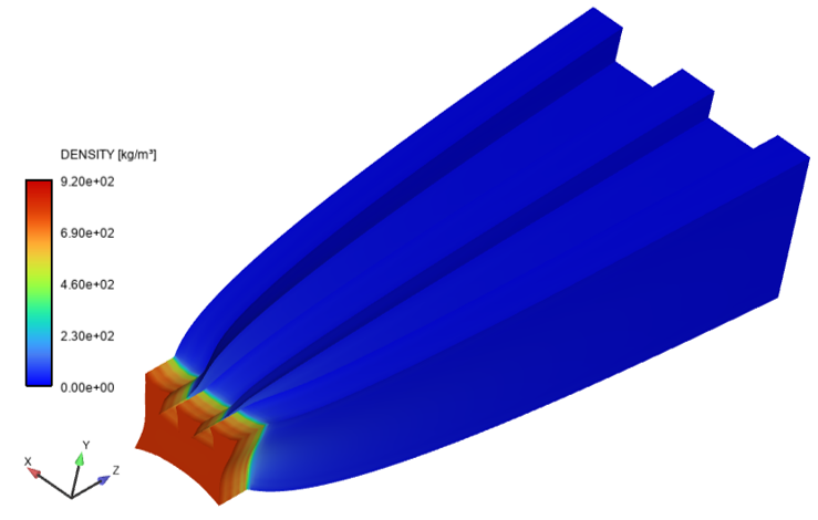
Figure 4.21: Die Lip Shape Determination for the Foamed Material displays the shape of the die lips that would be needed for extruding the desired extrudate profile for the foamed material. At first, you can see that the cross section of the die is significantly smaller than the initial section; the ratio of area cross sections is of about 1 to 7. This is a consequence of the foaming which essentially occurs after the material has exited the die. As expected, sharp angles are suggested in order to obtain the re-entrant corners of the profile. Also, you can observe the large cross-sections needed for obtaining the three horns of the profile. This is expected, since the average velocity in these regions is rather low. Of course, the calculated profile must be interpreted within the light of the selected rheological model and the slipping boundary conditions.
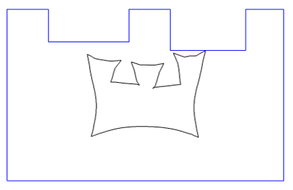
In Figure 4.21: Die Lip Shape Determination for the Foamed Material, the die profile is black while the required extrudate profile is blue.
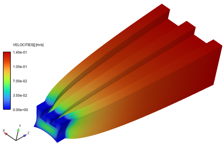
Another instructive result may be seen in Figure 4.22: Die Lip Shape Determination for the Foamed Material (Velocity Distribution) that displays the velocity distribution on the boundary of the computational domain as obtained at the end of the continuation scheme. As can be seen, the magnitude of the velocity is significantly larger for the foamed material (exit section of the extrudate) than for the dense material (inlet section of the die); in particular, the maximum value of the velocity is of about 0.14 m/s.
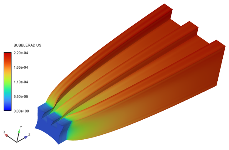
You can also examine the other calculated quantities. The first quantity is the bubble radius, which is displayed in Figure 4.23: Die Lip Shape Determination for the Foamed Material (Bubble Radius Distribution). As can be seen, the bubble radius increases from 0.027 mm (the value at the inlet) until approximately 0.22 mm at the exit of the calculation domain. In fact, the bubble radius exhibits a non-uniform distribution at the exit of the computational domain, ranging from approximately 0.16 to 0.22 mm, with an area-average value of about 0.17 mm. As suggested in Figure 4.22: Die Lip Shape Determination for the Foamed Material (Velocity Distribution), you can observe that the largest bubbles are found close to the three horns of the profile. Indeed, the long residence time of particles flowing in those regions allows for the significant growth of the bubbles.
This significant change of bubble radius is obviously accompanied by a visible change in the density of the foamed material. This is visible in Figure 4.24: Die Lip Shape Determination for the Foamed Material (Density Distribution) that displays the distribution of the density on the boundary of the domain. At the entry, you can identify the value of 790 kg/m3), while at the exit there is the density ranging between 10 and 25 kg/m3, with an average value of 22.5 kg/m3. The density ratio of the dense material to that of the foamed material is around 35. The calculation suggests that the bubble growth will cease beyond some distance with respect to the die exit. In actual industrial process, the limited amount of available foaming gas as well as thermal effects will obviously play a further role in bound the foaming.
This example is divided into the following sections:
This example demonstrates the simulation of the isothermal filling of a simple 2D part using the Volume of Fluid (VOF) technique. As a reminder, this technique offers a means of simulating a fluid flow with one or several free surfaces and is popular for injection and filling-type problems. The VOF technique uses a time-dependent approach, which is applied on a fixed mesh, that is, the kinematic condition is not tracked, and the simulation domain is not deformed or remeshed.
Theoretically, a drawback of such a technique is that the location where the zero-force condition is applied does not correspond to a region on which natural boundary conditions apply. Consequently, additional approximations are required, beyond those typically employed as part of the finite element method. Because of the explicit nature of VOF algorithms, a so-called Courant type of limitation always occurs, and the time step is limited to a fraction of the time it takes to transport information through an individual element (or cell). It is common to require hundreds of time steps to compute an entire simulation. Because each of these time steps are performed on a fixed domain with an inexpensive numerical technique, a VOF model can still require less CPU time than a simulation involving moving or deforming fluid domain, such as the Arbitrary Lagrangian-Eulerian (ALE) approach. The VOF model implemented here is intrinsically more robust than the ALE approach when modeling free surfaces that merge, separate, or are convoluted, and allows you to simulate problems that a deformation-based technique simply could not attack (for example, a complex cavity filling).
The volume of fluid method tracks a liquid fluid on a domain using material property variable, namely the fluid fraction. This variable is used to identify where the fluid is present, and is governed by a transport equation.
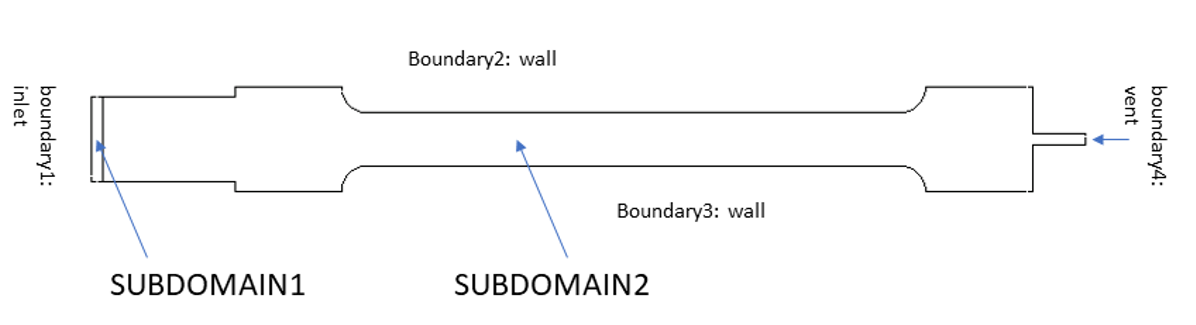
In the current example, consider the following material properties for the polymer, with ρ = 1000 kg/m3; η = 1000 Pa s. Inertia is taken into account. The geometry (see Figure 4.25: Geometry of the Test Sample ) is similar to a test sample generally used in traction tests. The width is 2cm and the total length is 20.5 cm. The cavity is empty at the start of the simulation. The inlet of the computation domain is Boundary1 with a volume flow of 1.5e-04 m3/s is imposed. The outlet is Boundary4 where a zero pressure is applied: it corresponds to a vent from where the air escapes from the cavity in the actual process (but not simulated) and from where some polymer will escape in the last stage of filling. The walls are defined by Boundary2 and Boundary3 where one can assume no slippage along the walls. The filling of the sample should last less than 20 seconds. The simulation will stop as soon as the cavity is filled.
The following sections describe the setup and solution steps for this example:
To prepare for running this example:
Download the
filling_sample.zipfile here .Unzip
filling_sample.zipto your working directory.The file,
filling_sample.msh, can be found in the folder.Use Fluent Launcher to start the Fluent Materials Processing workspace, with the Capability Level set to Enterprise.
Read in the mesh file.
![]() Setup → Read → Mesh...
Setup → Read → Mesh...
When reading the mesh file, the Define Mesh Unit dialog box appears where you can set the Mesh Length Unit to cm. Click Accept to apply the new setting and dismiss the dialog box.
For this example, choose a simulation template for filling. When using a template, the Fluent Materials Processing workspace creates a skeleton based on your choice, so that usually you only need to fill in the few fields. When using the template, you will note that under the General properties, the Calculation Type has been set to Volume of Fluid. To fulfill the setup, fluid material data must be provided, cell zones must be defined, and boundary conditions must be assigned. Eventually, solver options have to be selected before running the calculation.
![]() Setup → Simulation → Use
Template...
Setup → Simulation → Use
Template...
This displays the Simulation Template dialog box, where you can specify particular details for the type of simulation.
Set the Type to Filling.
Set the Number of Inlets to 1.
Set the Number of Vents to 1.
Set the Duration to 20 s.
Click Apply to close the dialog box. The workspace will set up the various requirements for the specified simulation type.
Define the material properties for the fluid.
![]() Setup → Materials →
fluid
Setup → Materials →
fluid
Expand the Density Law in the properties view.
Set the Density to 1000 kg/m3.
Expand the Viscosity Law in the properties view.
Set the Viscosity (of the Constant Law) to 1000 Pa s.
Define the cell zone properties for the fluid-zone.
![]() Setup → Cell Zones →
fluid-zone
Setup → Cell Zones →
fluid-zone
Set the Zones to include subdomain1 and subdomain2.
Define the conditions for the various boundaries in the simulation.
Define conditions at the inlet.
Setup → Fluid Boundary
Conditions → inletSet the Boundary Zone to boundary1.
Set the Flow Specification to Volume flow.
Set the Volume flow rate to 1.5e-4 m3/s.
Define conditions at the vent.
Setup → Fluid Boundary
Conditions → ventSet the Boundary Zone to boundary4.
Define conditions at the wall.
Setup → Fluid Boundary
Conditions → wallSet the Boundary Zone to boundary2-subdomain1, boundary2-subdomain2, boundary3-subdomain1, and boundary3-subdomain2.
Define any particular solution-based settings in the simulation.
Define any derived quantities.
Solution → Derived Quantities Review the pre-selected derived quantities.
Select any other quantities that are of interest.
Define any calculation activities.
Solution → Calculation
Activities Under Transient Controls, set the Initial Time Step to 0.1 s, the Minimum Time Step to 0.0001 s, the Maximum Time Step to 1 s, the Maximum Number of Steps to 1500, the Accuracy to 0.25, and the Filtering Threshold on Fluid Fraction to 0.1. The Stop Run When Cavity Full option should already be enabled.
Run the calculations.
The setup is now ready and it can now be checked, and the calculation can start.
Solution → Run Calculation Click Check to perform a final check of the setup and the coherence of the data.
If there are no errors or warnings, click Calculate. With the current mesh, the calculation requires approximately ten minutes, and 500 transient steps until completion.
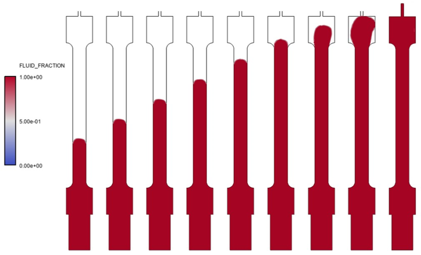
Figure 4.26: Fluid Fraction Contour (for Time = 0.1, 0.5, 1.0, 2.0, 3.0, 4.0, 5.0, 6.0, and 7.0 seconds) and Figure 4.27: Fluid Fraction Contour (for Time = 8.0, 9.0, 10.0, 11.0, 12.0, 13.0, 14.0, 15.0, and 15.84 seconds) show the progressive filling of the cavity. The time required to fill it up completely is 15.84 s and is coherent with its volume (actually surface) and the imposed flow rate.
Figure 4.26: Fluid Fraction Contour (for Time = 0.1, 0.5, 1.0, 2.0, 3.0, 4.0, 5.0, 6.0, and 7.0 seconds)
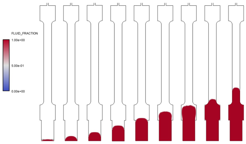
Figure 4.27: Fluid Fraction Contour (for Time = 8.0, 9.0, 10.0, 11.0, 12.0, 13.0, 14.0, 15.0, and 15.84 seconds)
This example is divided into the following sections:
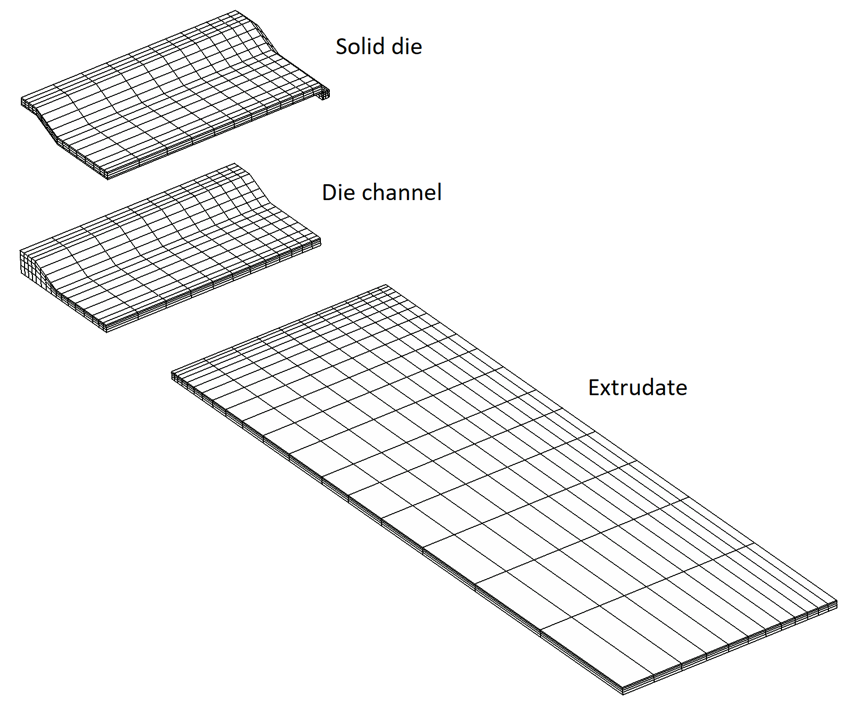
This example illustrates the Fluid Solid Interaction capability of the Fluent Materials Processing workspace by modeling the deformation of an extrusion die. Some dies do indeed deform, especially when extruding thin polymer sheet.
The geometry is depicted in Figure 4.28: Zones and consists of three zones - diechannel for the fluid in the die, extrudate for the free jet and soliddie for the steel die itself.
The different boundaries are shown in Figure 4.29: Boundaries .
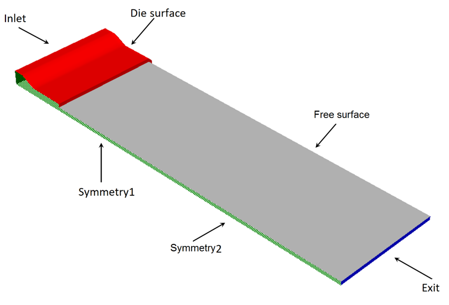
A flow rate Q is imposed at the inlet of the die channel, no slip conditions are applied on the wall of the die channel, an extrudate-exit is defined on the end of the free jet, symmetry conditions are imposed on the vertical and the horizontal planes of symmetry and a free border is defined on the steel die surface.
With SI units, the following numerical values are selected for the various data involved.
A flow rate of 3 x 10⁻⁷ m3/s is imposed at the inlet.
The viscosity of the Newtonian fluid is 10000 Pa s.
The Young modulus of the steel die is 2.1 x 10¹¹ Pa, while its Poisson coefficient is 0.3
Note that there is the assumption that inertia and gravity forces can be neglected.
The following sections describe the setup and solution steps for this example:
To prepare for running this example:
Download the
fsi3D.zipfile here .Unzip
fsi3D.zipto your working directory.The file,
fsi3D.msh, can be found in the folder.Use Fluent Launcher to start the Fluent Materials Processing workspace, with the Capability Level set to Enterprise.
Read in the mesh file.
![]() Setup → Read → Mesh...
Setup → Read → Mesh...
When reading the mesh file, the Define Mesh Unit dialog box appears where you can set the Mesh Length Unit to mm. Click Accept to apply the new setting and dismiss the dialog box.
For this example, choose a simulation template for extrusion. When using a template, the Fluent Materials Processing workspace creates a skeleton based on your choice, so that usually you only need to fill in the few fields. Typically, fluid material data need to be provided, cell zones must be defined, boundary conditions must be assigned, and the calculation of derived quantities must be activated as appropriate. Eventually, solver options have to be selected before running the calculation.
![]() Setup → Simulation → Use
Template...
Setup → Simulation → Use
Template...
This displays the Simulation Template dialog box, where you can specify particular details for the type of simulation.
Set the Type to Extrusion.
Set the Goal to Predict extrudate shape.
Click Apply to close the dialog box. The workspace will set up the various requirements for the specified simulation type.
Define the materials for the simulation.
Define the material properties for the fluid.
Setup → Materials →
fluid Expand the Viscosity Law in the properties view.
Set the Viscosity (of the Constant Law) to 10000 Pa s.
Add another material from the materials library. In this case, you will use the Ribbon, but you can also use the Outline View context menu or by clicking a button in the Properties View.
Setup → Materials →
Material → New → Import
from libraryThis displays the Library of Materials dialog box.
Set the Family to Miscellaneous.
Set the Material to Steel_Solid_300K.
Click OK to close the dialog box.
Check the properties for Solid Steel and confirm that under the material's Elastic Properties, the Young Modulus is 2.1e+11 Pa and that the Poisson Coefficient is set to 0.3.
Define cell zone properties for your simulation.
Define the cell zone properties for the fluid-zone.
Setup → Cell Zones →
fluid-zone Set the Zones to include diechannel and extrudate.
Add a new solid cell zone using the Ribbon.
Setup → Cell
Zones → Cell zone
→ New → Solid zoneSet the properties for the new solid cell zone (solid-zone-1)
Set the Zones to soliddie.
Set the Solid Model to Elastic.
Set the Solid Material to Solid Steel.
Define the conditions for the various boundaries in the simulation.
Define conditions at the extrudate-exit.
Setup → Fluid Boundary
Conditions → extrudate-exitSet the Boundary Zone to exit.
Define conditions at the free-surface.
Setup → Fluid Boundary
Conditions → free-surfaceSet the Boundary Zone to freesurface.
Set the Fixed Part to soliddie-diechannel (the die channel wall and the interface between the fluid and the steel die).
Define conditions at the inlet.
Setup → Fluid Boundary
Conditions → inletSet the Boundary Zone to inlet-diechannel.
Set the Flow Specification to Volume flow.
Set the Volume flow rate to 3.7e-7 m3/s.
Remove the extra wall fluid boundary condition (wall).
Setup → Fluid Boundary
Conditions → wallClick the Delete button to remove this particular condition.
Define a new fluid boundary condition (symmetry-1, using the Ribbon) and set its properties.
Setup → Boundary
Conditions → Fluid
→ New → SymmetrySet the properties for the new fluid boundary condition (symmetry-1)
Set the Boundary Zone to symmetry1-diechannel, and symmetry1-extrudate.
Define a new fluid boundary condition (symmetry-2, using the Ribbon) and set its properties.
Setup → Boundary
Conditions → Fluid
→ New → SymmetrySet the properties for the new fluid boundary condition (symmetry-2)
Set the Boundary Zone to symmetry2-diechannel, and symmetry2-extrudate.
Define a new solid boundary condition (free-1, using the Ribbon) and set its properties.
Setup → Boundary
Conditions → Solid
→ New → FreeSet the properties for the new solid boundary condition (free-1)
Set the Boundary Zone to diesurface.
Define a new solid boundary condition (symmetry-1, using the Ribbon) and set its properties.
Setup → Boundary
Conditions → Solid
→ New → SymmetrySet the properties for the new solid boundary condition (symmetry-1)
Set the Boundary Zone to symmetry1-soliddie, and symmetry2-soliddie.
Define a new solid boundary condition (normal-displacement-1, using the Ribbon) and set its properties.
Setup → Boundary
Conditions → Solid
→ New → Normal DisplacementSet the properties for the new solid boundary condition (normal-displacement-1)
Set the Boundary Zone to inlet-soliddie.
Set the Normal Displacement to 0 m.
Enable the Allow Non-Zero Tangential Displacement option.
Define a new interface boundary condition (fluid-solid-1, using the Ribbon) and set its properties.
Setup → Boundary
Conditions → Interface
→ New → Fluid-Solid
(conformal)Set the properties for the new interface boundary condition (fluid-solid-1)
Set the Interface Zone to soliddie-diechannel.
Define the conditions for the two mesh deformation regions.
Define the conditions on the extrudate.
Setup → Mesh Deformations
→ extrudateSet the Zones to extrudate.
Set the Inlet Section to extrudate-diechannel.
Set the Outlet Section to exit.
Define a new mesh deformation (extrudate-1, using the Ribbon) and set its properties.
Setup → Mesh
Deformations → Mesh deformation
→ New → ExtrudateSet the properties for the new mesh deformation (extrudate-1)
Set the Zones to diechannel.
Set the Inlet Section to inlet-diechannel.
Set the Outlet Section to extrudate-diechannel.
Define any particular solution-based settings in the simulation.
Define any derived quantities.
Solution → Derived Quantities Review the pre-selected derived quantities.
Select any other quantities that are of interest.
Define any calculation activities.
Solution → Calculation
Activities Under Convergence Strategies, enable both the Free Surfaces and Moving Interfaces and the Fluid-Structure Interaction (FSI) options.
Run the calculations.
The setup is now ready and it can now be checked, and the calculation can start.
Solution → Run Calculation Click Check to perform a final check of the setup and the coherence of the data.
If there are no errors or warnings, click Calculate.
In this example, it is assumed that you are already familiar the graphical analysis tools of the workspace. Figure 4.30: Displacement Contours on the Die Surface displays the magnitude of deformation on the outer surface of the steel die, while Figure 4.31: Displacement Vectors on the Die Channel Wall shows the deformation of the fluid-solid interface.
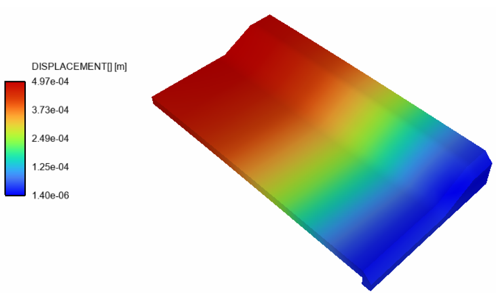
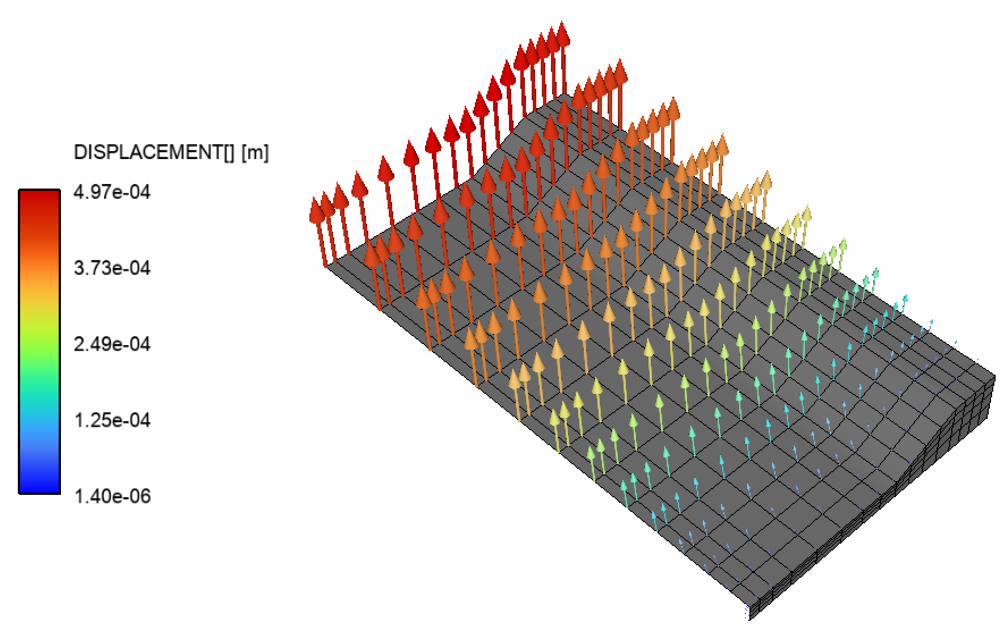
Figure 4.32: Die Lip compares the die lip before and after deformation (undeformed in yellow deformed in black).

Figure 4.33: Pressure Contours on the Fluid Domain displays the pressure drop in the die and allows you to visualize the shape of the free jet. Its deformation results from the velocity rearrangement after the die exit and the deformation of the die lip itself.
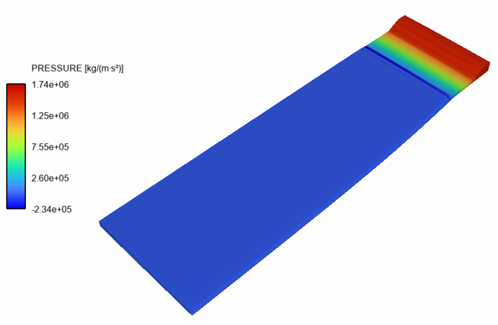
Lastly, Figure 4.34: Free Surface and Figure 4.35: Extrudate Exit compares the free surface and the extrudate final cross section with their shape before and after the calculation, the latter being also the initial die lip shape (undeformed in yellow deformed in black).
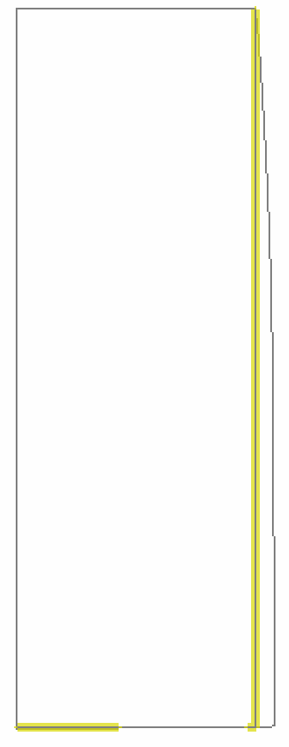

This example is divided into the following sections:
Internal flows of high-viscosity materials are often characterized by important pressure drops and temperature rise, the latter originating from viscous heating. The simulation of such internal flows can therefore be useful, for example, in order to evaluate the stresses that will be applied to a given flow device. This example demonstrates the thermal simulation of the internal flow of a high-viscosity fluid into a distributor with one inlet and four outlets. The pressure field is examined and one will note that the four outlet flow rates will not be identical, despite the apparent symmetry of the flow. Indeed, under well-known conditions, it can reasonably be assumed that the distribution of material is well balanced. However, geometric effects may affect the temperature distribution, and consequently, the ideal balance of material distribution is no longer guaranteed.
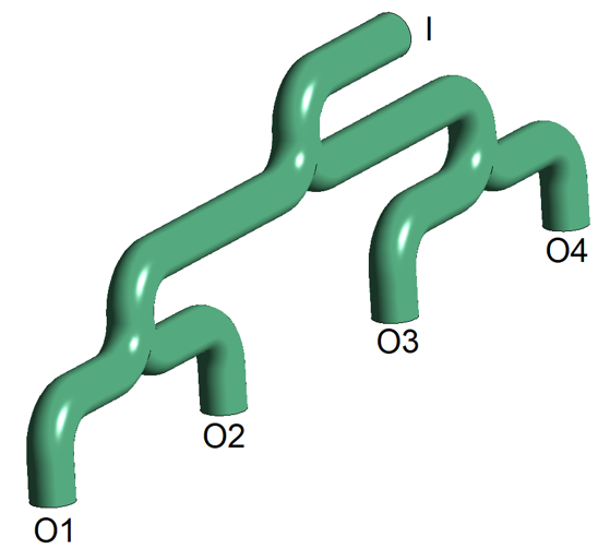
First consider the bifurcations channel as represented in Figure 4.36: Example of a Internal Flow , that consists of one inlet (I) and four outlets (O1 to O4). The box surrounding the geometry has the dimensions 88 x 26 x 4 mm. In particular, the radius of the channel is 2 mm. The path along the central geometric line is identical from the inlet to each outlet. However, when considering the paths close to the wall, differences are found, affecting the global flow, and consequently, the flow rates at the individual outlets.
One can assume that the fluid obeys the behavior of a generalized Newtonian material, and its shear-rate and temperature dependences of the viscosity are respectively described by means of the Bird-Carreau and Arrhenius laws, with the following parameters:
Shear-rate dependence: Bird-Carreau:
 = 104 Pa s,
  = 0.5 s, and n = 0.4
Arrhenius, vertical and horizontal shifts:
 = 3000 K,
  = 453.15 K
For the other parameters of the fluid, there are
density
 = 103 kg/m3
thermal conductivity k = 0.5 W/m/K
heat capacity
 = 2000 J/kg/K
Fluid enters through the inlet at a rate of 1.5x10‑6
m3/s, and with a temperature of 453.15 K. Standard outflow boundary
conditions are selected at all four exits. Slipping is imposed along the wall, and it obeys the
asymptotic law characterized by upper shear stress. Temperature dependence is defined on the
upper shear stress value and is described by the Arrhenius law. One can write the following
relationship for the tangential force  as a function of the tangential velocity
  and the temperature T:
 | (4–6) |
In this relationship, you can identify the asymptotic law for the dependence with respect to the tangential velocity: it actually bounds the tangential stress. You can also see the Arrhenius function for the temperature dependence, that suggests a decrease of the upper tangential stress limit when temperature increases. The following numerical values are selected for the several parameters:
k = 105 Pa,  = 0.002 m/s
 = 3000 K, and
  = 453.15 K
The following sections describe the setup and solution steps for this example:
To prepare for running this example:
Download the
Bifurcations.zipfile here .Unzip
Bifurcations.zipto your working directory.The file,
Bifurcations_channel.msh, can be found in the folder.Use Fluent Launcher to start the Fluent Materials Processing workspace, with the Capability Level set to Enterprise.
Read in the mesh file.
![]() Setup → Read → Mesh...
Setup → Read → Mesh...
When reading the mesh file, the Define Mesh Unit dialog box appears where you can set the Mesh Length Unit to m. Click Accept to apply the new setting and dismiss the dialog box.
For this example, choose a simulation template for internal flow. When using a template, the Fluent Materials Processing workspace creates a skeleton based on your choice, so that usually you only need to fill in the few fields. Typically, fluid material data need to be provided. Cell zones must be defined, boundary conditions must be assigned, and the calculation of derived quantities must be activated as appropriate. Eventually, solver options have to be selected before running the calculation.
![]() Setup → Simulation → Use
Template...
Setup → Simulation → Use
Template...
This displays the Simulation Template dialog box, where you can specify particular details for the type of simulation.
Set the Type to Internal Flow.
Enable the Thermal option.
Click Apply to close the dialog box. The workspace will set up the various requirements for the specified simulation type.
Define the thermal generatlized Newtonian material properties for the fluid.
![]() Setup → Materials →
fluid
Setup → Materials →
fluid
Expand the Density Law in the properties view.
Set the Density to 1000 kg/m3.
Expand the Thermal Properties in the properties view.
Set the Thermal Conductivity coefficient K to 0.5 W/(m K).
Set the Heat Capacity per Unit Mass coefficient Cp to 2000 J/(kg K).
Expand the Viscosity Law in the properties view.
Set the Shear Rate Dependence to Bird-Carreau.
Set the Temperature Dependence to Arrhenius .
Set the Zero Shear Viscosity to 10000 Pa s.
Set the Time Constant to 0.5 s.
Set the Power Law Index to 0.4.
Set the Ea/R to 3000 K.
Set the Reference Temperature to 453.15 K.
Set the Shift to Vertical and horizontal.
Define the cell zone properties for the fluid-zone.
![]() Setup → Cell Zones →
fluid-zone
Setup → Cell Zones →
fluid-zone
Set the Zones to include channel.
Set the Fluid Model to Generalized newtonian.
Set the Fluid Material(s) to fluid.
Define the conditions for the various boundaries in the simulation.
Define conditions at the inlet.
Setup → Fluid Boundary
Conditions → inletSet the Boundary Zone to inlet.
Set the Flow Specification to Volume flow.
Set the Incoming Material to fluid.
Set the Volume Flow Rate to 1.5e-6 m3/s.
Set the Temperature to 453.15 K.
Define conditions at the outlet.
Setup → Fluid Boundary
Conditions → outletSet the Boundary Zone to outlet1.
Set the Flow Specification to Pressure.
Set the Gauge Pressure to 0 Pa.
Under Thermal Condition, set the Option to Vanishing heat flux.
Add a new fluid boundary condition (outlet-2).
Setup → Fluid Boundary
Conditions New... Change the Name to outlet-2.
Set the Type to Outflow.
Set the Boundary Zone to include outlet2.
Set the Flow Specification to Pressure.
Set the Gauge Pressure to 0 Pa.
Under Thermal Condition, set the Option to Vanishing heat flux.
Add a new fluid boundary condition (outlet-3).
Setup → Fluid Boundary
Conditions New... Change the Name to outlet-3.
Set the Type to Outflow.
Set the Boundary Zone to include outlet3.
Set the Flow Specification to Pressure.
Set the Gauge Pressure to 0 Pa.
Under Thermal Condition, set the Option to Vanishing heat flux.
Add a new fluid boundary condition (outlet-4).
Setup → Fluid Boundary
Conditions New... Change the Name to outlet-4.
Set the Type to Outflow.
Set the Boundary Zone to include outlet4.
Set the Flow Specification to Pressure.
Set the Gauge Pressure to 0 Pa.
Under Thermal Condition, set the Option to Vanishing heat flux.
Define conditions at the wall.
Setup → Fluid Boundary
Conditions → wallSet the Boundary Zone to wall.
Set the Slip Specification to Partial slip.
Set the Slip Model to Asymptotic law .
Set the Friction Coefficient to 100000 Pa.
Set the Scaling Factor to 0.002.
Set the Temperature Dependence to Arrhenius law.
Set the Ea/R to 3000 K.
Set the Reference Temperature to 453.15 K.
Set the Wall Velocity to Stationary.
Under Thermal Condition, set the Option to Insulated.
Define any particular solution-based settings in the simulation.
Define the initial temperature.
Solution → Temperature
Initializations → temperature-in-fluid-zone Set the Cell Zones to fluid-zone.
Set the coefficient A to 453.15 K.
Define any calculation activities.
Solution → Calculation
Activities Set the Number of Processors to 4.
For Convergence Strategies, select Flow at Inlet.
Run the calculations.
The setup is now ready and it can now be checked, and the calculation can start.
Solution → Run Calculation Click Check to perform a final check of the setup and the coherence of the data.
If there are no errors or warnings, click Calculate. With the current mesh, the calculation requires approximately four minutes, and six continuation steps until completion.
In this example, it is assumed that you are already familiar the graphical analysis tools of the workspace.
Figure 4.37: Temperature Field on the Wall of the Flow Channel With One Inlet and Four Outlets displays the temperature distribution on the domain boundary, as obtained at the end of the calculation. The first striking observation is that one does not find a similar temperature development along the four branches of the flow domain. The rational for this is that the flow paths differ. At the first bifurcation, high wall temperature is convected on the upper part of the wall, while lower center temperature is convected on the lower part of the wall. A similar mechanism is found for the subsequent bifurcations. As a result, the highest temperature is found at the outside exits, while the inner exits exhibit a lower average temperature.
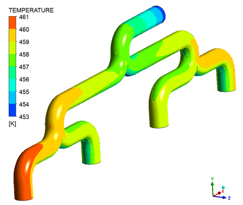
Figure 4.38: Temperature Field at all Four Outlets of the Flow Channel displays the temperature distributions at all four outlet sections. One can see that the outlet sections 1 and 4 exhibit the highest average temperature, respectively 457.6 and 457.2 K, while the outlet sections 2 and 3 exhibit the lowest average temperature, respectively 456.6 and 455.5 K. Also, to some extent, the distribution at each outlet is the fingerprint of the flow splitting. For example, a close inspection of the distribution at outlet 1 suggests that the fluid on the left-hand side has undergone the longest path, thus with the longest viscous heating, while the fluid on the right-hand side has undergone one flow splitting, at the last bifurcation. A similar comment can be made for the temperature distribution at outlet 4. For outlets 2 and 3, the average temperatures are lower, because the fluid that flows through them has mainly seen two stream splittings.
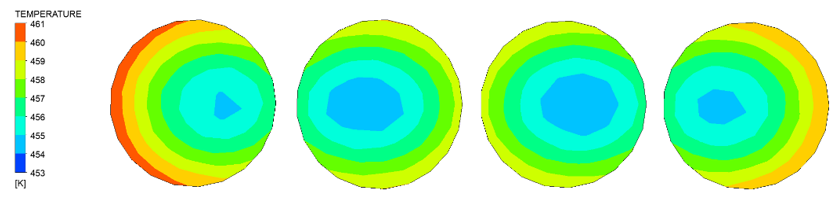
It is expected for all exit flow rates to be identical, for example, a quarter of the inlet flow rate. However, when viewing the temperature dependence of the viscosity, the flow distribution among the four exits is also affected. In the transcript, at the end of each continuation step, you can find the actual flow rate calculated along each boundary surface. When inspecting the values for the last continuation step, you will see that the flow rate at the second outlet is less than the flow rate at the first outlet and the flow rate at the third outlet is less than the flow rate at the fourth outlet. This is seen in Table 4.1: Relative Outlet Flow Rates at all Four Outlets which lists the ratio of all exit flow rates to the expected ideal one defined as a quarter of the inlet flow rate. You can see a relative difference of up to 6% between the flow rate at outlet 1 with respect to outlet 3.
Table 4.1: Relative Outlet Flow Rates at all Four Outlets
| Outlet | Relative Flow Rate (%) |
|---|---|
| 1 | 103.13 |
| 2 | 100.00 |
| 3 | 97.35 |
| 4 | 99.52 |
This example is divided into the following sections:
This example describes how to setup and solve a multi-layer film casting simulation where the rheology of the fluid layers is governed by multi-mode Double-Convected Pom-Pom models [DCPP] and the thermal effects are considered.
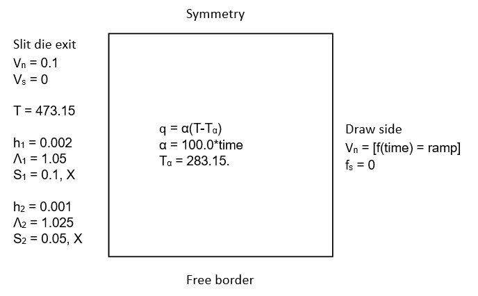
As shown in Figure 4.39: Example of a Multi-layer Film Casting ., the calculation domain is a square whose side length is 1 m. The other quantities are provided in the MKS system of units. As can be seen at first, next to velocity and thickness unknowns, temperature field is also calculated, since entry temperature and cooling are incorporated into the model. Here, it is considered that both fluid layers exit the slit die with an average velocity (V) of 0.1 m/s, and with a temperature (T) of 473.15 K. The thickness of both layers (h1, h2) is of 0.002 m and 0.001 m, respectively. Along the outlet section, a normal velocity of 0.8m/s is imposed. To help convergence, an expression is defined to make this velocity to progressively increase from 0.1 to 0.8 m/s.
A specific attribute of the DCPP model is that it involves the simultaneous calculation of macromolecular orientation and stretch. These quantities obey first-order differential equations and thus require boundary conditions at the inlet of the calculation domain, which describe the melt state when leaving the slit die of the film casting process. The present situation considers that the individual layers exhibit a moderate amount of anisotropy (S1, S2) and stretch (Λ1, Λ2) at the slit die exit.
The rheology of both fluid layers is described respectively with two and three modes. The
linear and non-linear data for both modes are listed in Table 4.2: Properties of Both Fluids: Material Parameters for the Multi-mode DCPP Model. For both fluid layers, a purely viscous component
( ) is added to the extra-stress tensor. Since cooling is involved in the present
calculation, the temperature dependence of the rheological properties is invoked, as well as
other relevant parameters. They are listed in Table 4.3: Properties of Both Fluids: Parameters for Momentum and Energy Equation.
) is added to the extra-stress tensor. Since cooling is involved in the present
calculation, the temperature dependence of the rheological properties is invoked, as well as
other relevant parameters. They are listed in Table 4.3: Properties of Both Fluids: Parameters for Momentum and Energy Equation.
Table 4.2: Properties of Both Fluids: Material Parameters for the Multi-mode DCPP Model
| Mode | Layer 1 | Layer 1 | |||
|---|---|---|---|---|---|
| 1 | 2 | 1 | 2 | 3 | |
| G [Pa] | 601 | 60.1 | 402 | 40.2 | 4.02 |
| [s] | 2.1 | 0.21 | 2.2 | 0.22 | 0.022 |
 [s] [s] | 0.81 | 0.081 | 0.82 | 0.082 | 0.0082 |
| q | 4.1 | 2.1 | 4.1 | 2.2 | 1.2 |
 | 0.151 | 0.251 | 0.252 | 0.262 | 0.272 |
| [Pa s] | 20.1 | 20.2 | |||
Table 4.3: Properties of Both Fluids: Parameters for Momentum and Energy Equation
| Layer 1 | Layer 1 | |
|---|---|---|
| Density: [kg/m3] | 1000 | 1100 |
| Heat Conductivity: k W/m/°C] | 0.5 | 0.55 |
| Heat Capacity: [J/kg/°C] | 2000 | 2300 |
| Activation Energy / R: | 4000 | 5000 |
| Ref. Temperature: [°C] | 473.15 | 473.15 |
For performing the numerical simulation, the mesh shown in Figure 4.40: Film Casting: Finite Element Mesh is used, and it is characterized by 180 elements, with small elements in the vicinity of the starting point of the free border.
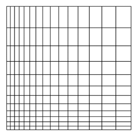
Streamline upwinding is used for integrating the convective terms in the constitutive and energy equations, as well as for integrating the kinematic equation of the free border. As shown in Figure 4.39: Example of a Multi-layer Film Casting , evolution schemes are applied on the take-up velocity as well as on the heat transfer coefficient. A linear function is applied to the heat transfer coefficient, while a ramp function is applied on the take-up velocity which increases from 0.1 to 0.8:
 | (4–7) |
Stretching and anisotropy boundary conditions
For the case of the DCPP model used within a film casting simulation, care is required when imposing the boundary conditions for the viscoelastic variables at the inlet of the calculation domain. The inlet is identified as the border where the thickness condition is imposed. Here, instead of imposing values for all components of the orientation tensor, anisotropy described in terms of orientation and factor is given, as well as stretching amplitude. Imposing boundary conditions for the viscoelastic unknowns (orientation and stretching) is optional. If conditions are imposed, three data are required:
the direction of anisotropy of the orientation tensor (x or y),
the anisotropy factor ranging between 0 (isotropic) and 1 (anisotropic),
the inlet stretching.
By default, the anisotropy direction is along the x-axis, the anisotropy factor is 0, while the stretching is 1. This corresponds to a situation where the melt has not undergone deformation in the die before being extended in the film drawing. Actually, the flow in a die is dominated by shear, which may certainly affect the orientation tensor, while stretching will remain close to unity. Therefore, a typical inlet boundary condition for film casting would involve a non-zero anisotropy factor and a unit stretching. You can change this according to your needs.
On the basis of the value entered for the anisotropy direction and anisotropy factors, the value of the orientation tensor S at the inlet can be evaluated and assigned as Saa=(2s+1)/3, Sbb=Szz=(1-s)/3 (where a is the selected direction of anisotropy, while b is perpendicular to it in the plane of the film). The component Sxy=0. If s=0 (isotropic), all three components of S are set to 1/3. If s=1 (100% anisotropy), then Saa=1, while the other components vanish. Any value between 0 and 1 is valid.
For the stretching variable, recommended values should be at least equal to unity. Values lower than unity are of course permitted but would probably not match the physics undergone in the die.
When a multi-layer system is defined, inlet boundary conditions can be defined independently for each layer, as it is already the case for the thickness. In the case of multi-mode model for a given layer, all modes will undergo the same selected inlet conditions.
Stress condition at the inlet of the calculation domain
It is worth mentioning that the solver exhibits better performances when reasonable inlet boundary conditions are selected for the viscoelastic unknowns of the DCPP model in film casting. Some situations have been reported to perform better when stresses are not imposed at the inlet of the calculation domain. In particular, this is the case when the rheology does not involve any additional purely viscous component.
The following sections describe the setup and solution steps for this example:
To prepare for running this example:
Download the
Film_VE.zipfile here .Unzip
Film_VE.zipto your working directory.The file,
Film_VE.msh, can be found in the folder.Use Fluent Launcher to start the Fluent Materials Processing workspace, with the Capability Level set to Enterprise.
Read in the mesh file.
![]() Setup → Read → Mesh...
Setup → Read → Mesh...
When reading the mesh file, the Define Mesh Unit dialog box appears where you can set the Mesh Length Unit to m. Click Accept to apply the new setting and dismiss the dialog box.
For this example, choose a simulation template for film casting. When using a template, the Fluent Materials Processing workspace creates a skeleton based on your choice, so that usually you only need to fill in the few fields. Typically, fluid material data for each layer need to be provided. Cell zones must be defined, boundary conditions must be assigned, mesh deformations must be defined, and the calculation of derived quantities must be activated as appropriate. Eventually, solver options have to be selected before running the calculation.
![]() Setup → Simulation → Use
Template...
Setup → Simulation → Use
Template...
This displays the Simulation Template dialog box, where you can specify particular details for the type of simulation.
Set the Type to Film Casting.
Set the Number of Layers to 2.
Enable the Thermal option.
Click Apply to close the dialog box. The workspace will set up the various requirements for the specified simulation type.
Define some general properties for the simulation.
![]() Setup → General
Setup → General
Set the Calculation Type to Continuation.
Define the thermal differential viscoelastic material properties for first layer (fluid-1).
![]() Setup → Materials →
fluid-1
Setup → Materials →
fluid-1
Expand the Density Law in the properties view.
Set the Density to 1000 kg/m3.
Expand the Thermal Properties in the properties view.
Set the Thermal Conductivity property K to 0.5 W/(m K).
Set the Heat Capacity per Unit Mass property Cp to 2000 J/(kg K).
Expand the Differential Viscoelastic Properties in the properties view.
Set the Model to POMPOM.
Set the Number of Relaxation Modes to 2 .
Set the Additional Viscosity to 20.1 Pa s.
Under Mode 1:
Set the Relaxation Time for Reorientation to 2.1 s.
Set the Relaxation Time for Stretching to 0.81.
Set the Shear Modulus to 601 Pa.
Set the Number of Arms to 4.1.
Set the Xi to 0.151.
Under Mode 2:
Set the Relaxation Time for Reorientation to 0.21 s.
Set the Relaxation Time for Stretching to 0.081.
Set the Shear Modulus to 60.1 Pa.
Set the Number of Arms to 2.1.
Set the Xi to 0.251.
Under Thermal Dependency:
Set the Temperature Dependence to Arrhenius.
Set the Ea/R to 4000 K.
Set the Reference Temperature to 453.15 K.
Define the thermal differential viscoelastic material properties for second layer (fluid-2).
![]() Setup → Materials →
fluid-2
Setup → Materials →
fluid-2
Expand the Density Law in the properties view.
Set the Density to 1100 kg/m3.
Expand the Thermal Properties in the properties view.
Set the Thermal Conductivity property K to 0.55 W/(m K).
Set the Heat Capacity per Unit Mass property Cp to 2300 J/(kg K).
Expand the Differential Viscoelastic Properties in the properties view.
Set the Model to POMPOM.
Set the Number of Relaxation Modes to 3 .
Set the Additional Viscosity to 20.2 Pa s.
Under Mode 1:
Set the Relaxation Time for Reorientation to 2.2 s.
Set the Relaxation Time for Stretching to 0.82.
Set the Shear Modulus to 402 Pa.
Set the Number of Arms to 4.2.
Set the Xi to 0.252.
Under Mode 2:
Set the Relaxation Time for Reorientation to 0.22 s.
Set the Relaxation Time for Stretching to 0.082.
Set the Shear Modulus to 40.2 Pa.
Set the Number of Arms to 2.2.
Set the Xi to 0.262.
Under Mode 3:
Set the Relaxation Time for Reorientation to 0.022 s.
Set the Relaxation Time for Stretching to 0.0082.
Set the Shear Modulus to 4.02 Pa.
Set the Number of Arms to 1.2.
Set the Xi to 0.272.
Under Thermal Dependency:
Set the Temperature Dependence to Arrhenius.
Set the Ea/R to 5000 K.
Set the Reference Temperature to 473.15 K.
Define the cell zone properties for the fluid-zone.
![]() Setup → Cell Zones →
fluid-zone
Setup → Cell Zones →
fluid-zone
Set the Zones to include subdomain1.
Set the Fluid Model to Differential viscoelastic.
Set the Surface Heat Source to Convection.
Set the Heat Transfer Coefficient to expression and enter 100*time W/(m2 K).
Set the Convection Temperature to 283.15 K.
Define the properties for the various layers in the simulation.
Define layer properties for layer-of-fluid-1.
Setup → Layers →
layer-of-fluid-1Set the Zones to include boundary4.
Set A to 0.002 m.
Enable Stress Condition Activation.
Set Direction of Anisotropy to X.
Set Anisotropy Factor to 0.1.
Set Stretching to 1.05.
Define layer properties for layer-of-fluid-2.
Setup → Layers →
layer-of-fluid-2Set the Zones to include boundary4.
Set A to 0.001 m.
Select Stress Condition Activation.
Set Direction of Anisotropy to X.
Set Anisotropy Factor to 0.05.
Set Stretching to 1.025.
Define the conditions for the various boundaries in the simulation.
Define fluid boundary conditions at the inlet.
Setup → Fluid Boundary
Conditions → inletSet the Boundary Zone to boundary4.
Under Inflow Condition:
Set the Normal Velocity to 0.1 m/s.
Deselect the Allow Non-Zero Tangential Velocity option.
Under Thermal Condition:
Set the Option to Temperature.
Set the Temperature to 473.15 K.
Define conditions at the outlet.
Setup → Fluid Boundary
Conditions → outletSet the Boundary Zone to boundary2.
Under Outflow Condition:
Set the Flow Specification to Velocity.
Set the Normal Velocity drop-down menu to expression, and enter the following: IF(time <= 0, 0.1, IF(time >= 1, 0.8, 0.1 + 0.7 * time)).
Select the Allow Non-Zero Tangential Velocity option.
Under Thermal Condition, set the Option to Vanishing heat flux.
Define conditions for free-surface-1.
Setup → Fluid Boundary
Conditions → free-surface-1Set the Boundary Zone to boundary1.
Under Free Surface Condition:
Set the Fixed Part to boundary4.
Set the Direction of Displacement to Y.
Under Thermal Condition, set the Option to Insulated.
Define conditions for free-surface-2.
Setup → Fluid Boundary
Conditions → free-surface-2Change the Name to Symmetry.
Set the Type to Symmetry.
Set the Boundary Zone to boundary3.
Define the conditions for the various mesh deformations in the simulation.
Set the conditions for the fluid deformation.
Setup → Mesh Deformations
→ fluid-deformationSet the Zones to subdomain1.
Set the Inlet Section to boundary4.
Set the Outlet Section to boundary2.
Define any particular solution-based settings in the simulation.
Define the initial temperature.
Solution → Temperature
Initializations → temperature-in-fluid-zone Set the Cell Zones to fluid-zone.
Set the coefficient A to 473.15 K.
(optional) Define a probe for the lower right side of the domain.
Solution →
Probes New... Set the Name to Neck.
Set the X to 1.
Set the Mode to moving node.
(optional) Define a probe for the upper right side of the domain.
Solution →
Probes New... Set the Name to Symm.
Set the X to 1.
Set the Y to 1.
Set the Mode to fixed geometric location.
Define any calculation activities.
Solution → Calculation
Activities Set the Number of Processors to 4.
Set the Initial Step Size to 0.01.
Define the outputs.
Solution → Outputs Set the Fields Visualization to Standard + special fields.
Run the calculations.
The setup is now ready and it can now be checked, and the calculation can start.
Solution → Run Calculation Click Check to perform a final check of the setup and the coherence of the data.
If there are no errors or warnings, click Calculate.
Ten continuation steps are needed for reaching the desired take-up velocity. In particular, the first continuation steps involve a relatively small step, which eventually increases until the upper-limit is reached.
In this example, some graphical analysis tools will be set up to assist in studying the results of the simulation. Of interest in this example are the simulation results as obtained at the end of the continuation scheme when the required take-up velocity is reached as well as the required heat flux on the film surface.
Define graphics LIC settings.
Results → Graphics
→ LIC SettingsSet the Vector Field to VELOCITIES.
Define contour plots of horizontal velocity.
Results → Graphics
→ Contours New...Set the Name to Horizontal Velocity.
Set the Field to VELOCITY[X].
Set the Surfaces to subdomain1.
Select the Contour Lines option.
Deselect the Auto-Compute Range option.
Set the Minimum Value to 0.1 m/s.
Expand the Color Map settings and set the Size to 20.
Click the Display button to see the contour plot in the Graphics window.
Figure 4.41: Contours of Velocities displays the horizontal velocity distribution at the end of the continuation scheme. As can be seen, it starts from 0.1 and increases until the assigned value of 0.8. Also, this result shows the shape of the film as well with the resulting neck-in. It is important to note that both fluid layers obey a unique velocity field and undergo thus the same shape deformation.
Define contour plots of temperature.
Results → Graphics
→ Contours New...Set the Name to Temperature.
Set the Field to TEMPERATURE.
Set the Surfaces to subdomain1.
Select the Contour Lines option.
Expand the Color Map settings:
Set the Size to 20.
Set the Precision to 4.
Click the Display button to see the contour plot in the Graphics window.
Figure 4.42: Contours of Temperature displays the temperature distribution obtained at the end of the continuation scheme. It shows a decrease of about 20.7 °K. The temperature field is also unique for both fluid layers.
Define contour plots of the first layer thickness.
Results → Graphics
→ Contours New...Set the Name to Thickness Layer-1.
Set the Field to THICKNESS_1.
Set the Surfaces to subdomain1.
Select the Contour Lines option.
Under Range:
Deselect the Auto-Compute Range option.
Set the Minimum Value to 0.0 m.
Set the Maximum Value to 0.002 m.
Expand the Color Map settings and set the Size to 20.
Click the Display button to see the contour plot in the Graphics window.
Define contour plots of the second layer thickness.
Results → Graphics
→ Contours →
Thickness-Layer-1 Copy...Change the Name to Thickness Layer-2.
Change the Field to THICKNESS_2.
Under Range:
Set the Minimum Value to 0.0 m.
Set the Maximum Value to 0.002 m.
Click the Display button to see the contour plot in the Graphics window.
Each fluid layer carries its own thickness distribution. Figure 4.43: Contours of Thickness (1) and Figure 4.44: Contours of Thickness (2) display the thickness distribution of each layer, obtained at the end of the continuation scheme. As can be seen, the thickness decreases along the horizontal direction. In the present situation, both thickness distributions exhibit a similar development. This originates from the fact that they start with uniform boundary conditions at the inlet to the calculation domain, with different values. As is typical in film casting, the thickness distribution exhibits higher values along the free border; in the literature this is referred to as edge-beading or dog-bone effect. It is interesting to note that the thickness distributions are essentially free of oscillations.
Define contour plots of the first layer extra stress.
Results → Graphics
→ Contours New...Set the Name to st11 Layer-1.
Set the Field to STRESSES_1_XX.
Set the Surfaces to subdomain1.
Select the Contour Lines option.
Under Range:
Deselect the Auto-Compute Range option.
Set the Minimum Value to 0.0 Pa.
Set the Maximum Value to 5500 Pa.
Expand the Color Map settings and set the Size to 20.
Click the Display button to see the contour plot in the Graphics window.
Define contour plots of the second layer extra stress.
Results → Graphics
→ Contours → st11
Layer-1 Copy...Change the Name to st11 Layer-2.
Change the Field to STRESSES_2_XX.
Under Range:
Set the Minimum Value to 0.0 Pa.
Set the Maximum Value to 5500 Pa.
Click the Display button to see the contour plot in the Graphics window.
Eventually, it is interesting to examine the development of the extra-stress component along the horizontal direction (corresponding to the stretching). Since each layer is characterized by its individual rheology, each layer also sees its own stress development. Figure 4.45: Contours of Extra Stresses (Layer 1) and Figure 4.46: Contours of Extra Stresses (Layer 2) display the distribution of the extra-stress component along the stretching direction, for both layers. As can be observed, the stress-component increases along the stretching direction; this results from the simultaneous neck-in and thickness decrease.
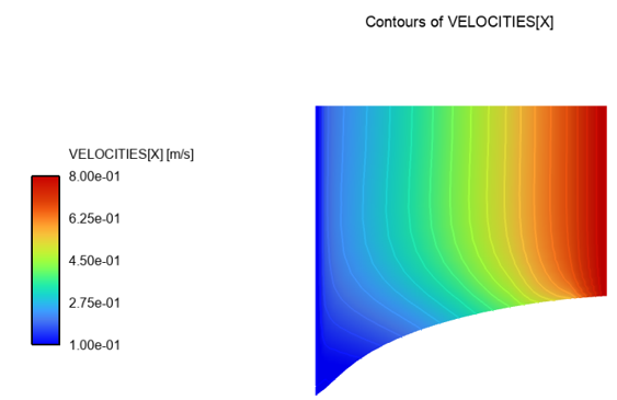
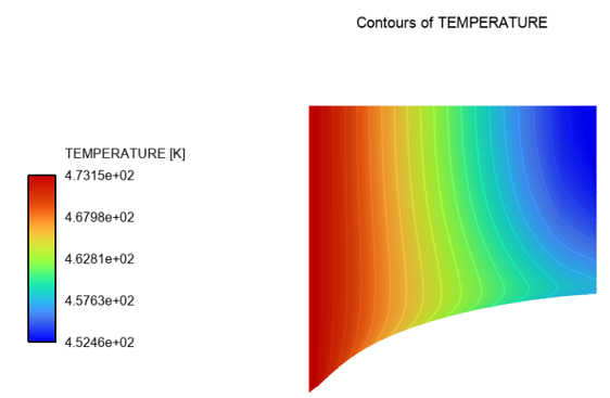
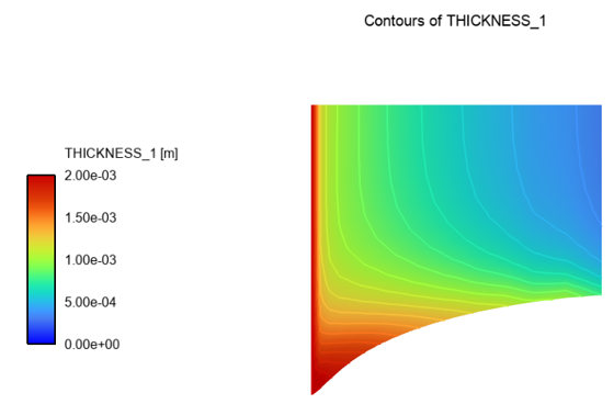
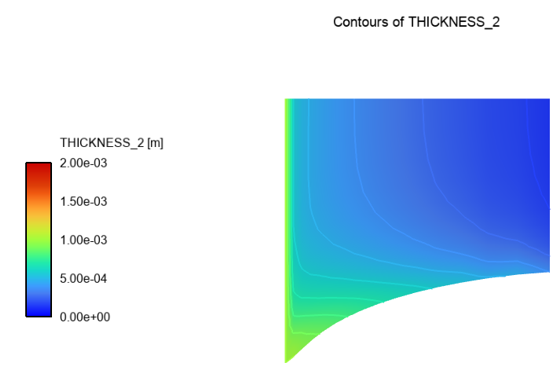
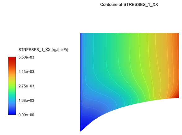
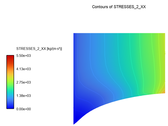
This example is divided into the following sections:
You will simulate the 3D non-isothermal extrusion of a rubber profile reinforced with a metal insert in this example. The heat transfer that occurs between the extruded rubber and the moving insert is the focus. Because rubber has a high viscosity, the heat effect may play a visible part in the process. Consider a small-sized object reinforced with a flat n-shaped metal insert as an example. The flow simulation including conjugated heat transfer with a moving element does not include any special difficulties: it is a steady simulation in which convection is added to the heat conduction problem for the metal insert.
The computational domain for the fluid and the metal insert is shown in Figure 4.47: 3D Non-isothermal Extrusion of a Rubber Profile Reinforced With a Metal Insert. Left: Calculation Domain With Die Region (Blue), Extrudate (Light Blue), Metal Insert (Grey). Right Above: Open View of the Domain. Right Below: Boundaries With, From Left to Right, Inlet (Orange), Die Wall (Blue), Interface With Metal Insert (Grey), Extrudate Wall (Light Blue), Outlet (Light Orange). Geometrically, the computation domain is encompassed by a box with dimensions of 13 x 4.3 x 50 mm.
Figure 4.47: 3D Non-isothermal Extrusion of a Rubber Profile Reinforced With a Metal Insert. Left: Calculation Domain With Die Region (Blue), Extrudate (Light Blue), Metal Insert (Grey). Right Above: Open View of the Domain. Right Below: Boundaries With, From Left to Right, Inlet (Orange), Die Wall (Blue), Interface With Metal Insert (Grey), Extrudate Wall (Light Blue), Outlet (Light Orange)
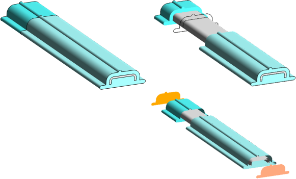
The calculation domain involves two subdomains, a rubber flow (inside the die and in the free jet), and a subdomain for the metal insert. Boundaries and boundary conditions are explained as follows: the rubber enters the domain with a flow rate of 1500 mm3/s (1.5 E-6 m3/s) and a temperature of 110 °C, while the metal insert enters with a velocity of 40 mm/s (0.04 m/s) and a temperature of 50 °C. The rubber slips along the die wall and the metal insert. It is assumed that the slipping obeys the asymptotic law with an upper shear stress value of 0.4 MPa and a critical velocity parameter of 1 mm/s (0.001 m/s). The velocity of the metal insert is considered at the interface. It is also assumed that the die temperature is controlled via a heat transfer coefficient of 200 W/m2/°C with a distant temperature of 60 °C. We also assume that the extrudate is rapidly cooled down into water, and that the heat exchange is described via a heat transfer coefficient of 1000 W/m2/°C with a distant temperature of 20 °C. Eventually, usual conditions are imposed at the interface between the rubber and the metal insert.
Consider the following data for rubber material qualities. For rheology, it is assumed that the shear-rate and temperature dependences of viscosity obey the Bird-Carreau and Arrhenius laws, respectively:
 | (4–8) |
with
 | (4–9) |
 | (4–10) |
You also have
 | (4–11) |
 | (4–12) |
 | (4–13) |
For the metal insert, only properties involved into the energy equation are needed:
 | (4–14) |
 | (4–15) |
 | (4–16) |
The discretization for the rubber domain and the metal insert is shown in Figure 4.48: Finite Element Discretization. The rubber region's finite element mesh has around 27000 hex and wedge elements, whereas the metal insert has approximately 8800 hex elements.
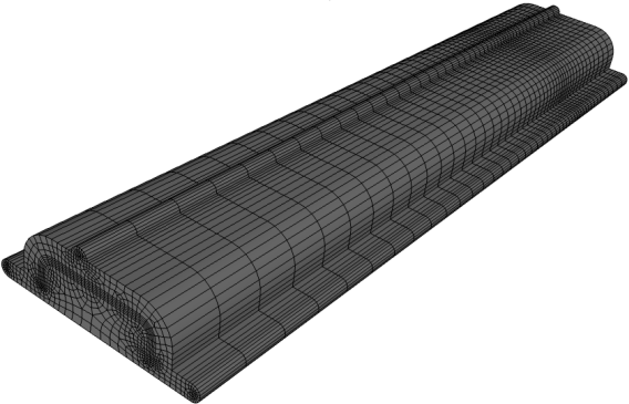
In this example, you will utilize the Extrusion Type Simulation Template using the Predict extrudate shape Goal to build the majority of the objects required for the simulation.
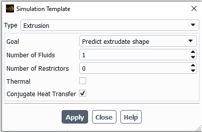
You must provide the density and viscosity law of the polymer matrix under
![]() Setup → Materials →
fluid.
Setup → Materials →
fluid.
Then, like with any extrusion simulation, provide the boundary conditions.
Data for the mesh deformations for the extrudate should be updated. The adaptive-die-section object (created by the template but irrelevant in this example) should be deleted.
Finally, activate the convergence algorithms to handle all of the non-linearities in this simulation such free surfaces and moving interfaces, viscosity and slip, and foaming.
The following sections describe the setup and solution steps for this example:
To prepare for running this example:
Download the
metal_insert.zipfile here .Unzip
metal_insert.zipto your working directory.The file,
metal_insert.poly, can be found in the folder.Use Fluent Launcher to start the Fluent Materials Processing workspace, with the Capability Level set to Enterprise.
Select an extrusion simulation template for this example. When you choose a template, the Fluent Materials Processing workspace generates a skeleton based on your selection, so you typically only need to fill up a few fields. Typically, fluid material data must be supplied. Cell zones must be created, boundary constraints provided, and a mesh deformation method (for extrudate section) specified. Before conducting the calculation, solver options must be selected.
![]() Setup → Simulation → Use
Template...
Setup → Simulation → Use
Template...
This displays the Simulation Template dialog box, where you can specify particular details for the type of simulation.
Set the Type to Extrusion.
Set the Goal to Predict extrudate shape.
Enable the Conjugate Heat Transfer option.
Click Apply to close the dialog box. The workspace will set up the various requirements for the specified simulation type.
Define the material properties for the fluid.
![]() Setup → Materials →
fluid
Setup → Materials →
fluid
Expand the Thermal Properties in the properties view.
Set the Thermal Conductivity property K to 0.5 W/(m K).
Set the Heat Capacity per Unit Mass property Cp to 2000 J/(kg K).
Expand the Viscosity Law in the properties view.
Set the Shear Rate Dependence to Bird-Carreau.
Set the Temperature Dependence to Arrhenius.
Set the Zero Shear Viscosity to 1000000 Pa s.
Set the Time Constant to 10 s.
Set the Power Law Index to 0.2.
Set Ea/R to 2500 K.
Set the Reference Temperature to 383 K.
Define the material properties for the solid.
![]() Setup → Materials →
solid
Setup → Materials →
solid
Expand the Density Law in the properties view.
Set the Density to 7500 kg/m3.
Expand the Thermal Properties in the properties view.
Set the Thermal Conductivity property K to 100 W/(m K).
Set the Heat Capacity per Unit Mass property Cp to 1000 J/(kg K).
Define the cell zone properties for the fluid-zone.
![]() Setup → Cell Zones →
fluid-zone
Setup → Cell Zones →
fluid-zone
Set the Zones to include die and extr.
Define the cell zone properties for the solid-zone.
![]() Setup → Cell Zones →
solid-zone
Setup → Cell Zones →
solid-zone
Set the Zones to include insert.
Enable Activation under Solid Motion.
Set Vz to 0.04 m/s.
Define the fluid boundary conditions.
Define fluid boundary conditions at the extrudate-exit.
Setup → Fluid Boundary
Conditions → extrudate-exitSet the Boundary Zone to outlet-extr.
Define conditions for free-surface.
Setup → Fluid Boundary
Conditions → free-surfaceSet the Boundary Zone to frees.
Set the Fixed Part to wall (the attachment line of the free surface).
Set the Thermal Condition to Convection.
Set the Heat Transfer Coefficient to 1000 W/(m2 K).
Set the Convection Temperature to 293 K.
Define conditions at the inlet.
Setup → Fluid Boundary
Conditions → inletSet the Boundary Zone to inlet-die.
Set the Flow Specification to Volume flow.
Set the Method to Computed dynamically to compute the inflow in the same solver sequence as the main flow.
Set the Volume flow rate to 1.5e-6 m3/s.
Set the Temperature to 383 K.
Define a new fluid boundary condition.
Setup → Boundary Conditions
→ Fluid → New →
WallChange the Name to wall.
Set the Boundary Zone to wall.
Set the Slip Specification to Partial slip.
Set the Slip Model to Asymptotic law.
Set the Friction Coefficient to 400000 Pa.
Set the Scaling Factor to 0.001 m/s.
Set Thermal Condition to Convection.
Set the Heat Transfer Coefficient to 200 W/(m2 K).
Set the Convection Temperature to 333 K.
Define the solid boundary conditions.
Define a new solid boundary condition.
Setup → Boundary Conditions
→ Solid → New →
TemperatureChange the Name to inlet.
Set the Boundary Zone to inlet-insert.
Set the Temperature to 323 K.
Define a new solid boundary condition.
Setup → Boundary Conditions
→ Solid → New →
InsulatedChange the Name to outlet.
Set the Boundary Zone to outlet-insert.
Define the interface boundary conditions.
Define condition at the interface.
Setup → Interface Boundary
Conditions → fluid-solid-interfaceSet the Interface Zone to insert-die and insert-extr.
Set the Wall Condition to Partial slip.
Set the Slip Model to Asymptotic law.
Set the Friction Coefficient to 400000 Pa.
Set the Scaling Factor to 0.001 m/s.
Define the conditions for the various mesh deformations in the simulation.
Define the mesh deformation conditions for the extrudate.
Setup → Mesh Deformations
→ extrudateSet the Zones to extr.
Set the Extrudate Deformation Method to Elastic.
Set the Inlet Section to extr-die.
Set the Outlet Section to outlet-extr.
Set the No Displacement on Section to insert-extr.
Define any particular solution-based settings in the simulation.
Define the initial temperature.
Solution → Temperature
Initializations → temperature-in-fluid-zone Set the coefficient A to 383 K.
Define the initial temperature.
Solution → Temperature
Initializations → temperature-in-solid-zone Set the coefficient A to 323 K.
Define the derived quantities.
Solution → Derived Quantities Select any quantities that are of interest.
Decouple the temperature calculation.
Solution → Methods Enable the Decouple Computation of Temperature.
Define any calculation activities.
Solution → Calculation
Activities Set the Solver Type to AMF direct solver + secant (as the decoupling of the temperature calculation will increase the number of iterations, one chooses cheaper iterations).
For Convergence Strategies, select Free Surfaces and Moving Interfaces, Viscosity and Slip and Thermal Effects.
Run the calculations.
The setup is now ready and it can now be checked, and the calculation can start.
Solution → Run Calculation Click Check to perform a final check of the setup and the coherence of the data.
If there are no errors or warnings, click Calculate.
With the current mesh, the calculation takes around an hour and six continuation steps to complete.
The calculation of the solution is relatively straightforward when using convergence algorithms.
In Figure 4.49: Velocity Magnitude on Outer Boundaries (Left) and on Some Cutting Planes and on the Metal Insert (Right), the velocity contours on the outer boundaries of the calculation domain are shown, and on the other side, the velocity contours on several cross-section planes (Z=-0.01 (inlet), -0.005, 0.000 (die exit), 0.005, 0.0125, 0.023, and 0.04 (extrudate exit)) and the metal insert are shown.
Figure 4.49: Velocity Magnitude on Outer Boundaries (Left) and on Some Cutting Planes and on the Metal Insert (Right)
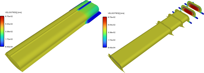
Figure 4.50: Contours of Local Shear-Rate on Outer Boundaries (Left) and on Some Cutting Planes and on the Metal Insert (Right) displays local shear-rate contours on the same surfaces as Figure 4.49: Velocity Magnitude on Outer Boundaries (Left) and on Some Cutting Planes and on the Metal Insert (Right)
Figure 4.50: Contours of Local Shear-Rate on Outer Boundaries (Left) and on Some Cutting Planes and on the Metal Insert (Right)
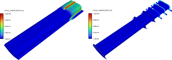
Figure 4.51: Contours of Viscosity on Outer Boundaries (Left) and on Some Cutting Planes and on the Metal Insert (Right) shows rubber viscosity contours on the same surfaces as the prior images.
Figure 4.51: Contours of Viscosity on Outer Boundaries (Left) and on Some Cutting Planes and on the Metal Insert (Right)
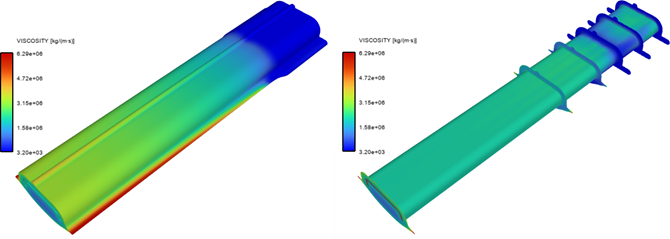
Figure 4.52: Contours of Temperature on Outer Boundaries (Left) and on Some Cutting Planes and on the Metal Insert (Right) displays the temperature contours.
Figure 4.52: Contours of Temperature on Outer Boundaries (Left) and on Some Cutting Planes and on the Metal Insert (Right)
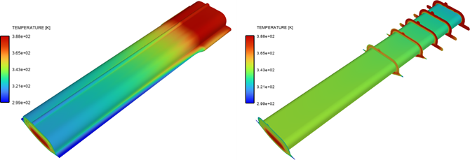
Figure 4.53: Contours of Temperature in Planes Cutting the Metal Insert shows temperature contours appearing on a series of cross-sections with a spacing of 5 mm.
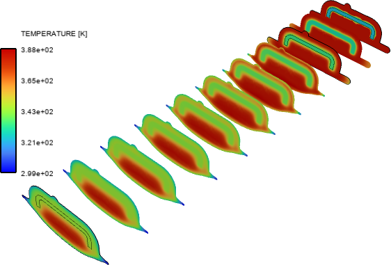
This example is divided into the following sections:
Profile extrusion is sometimes assisted by a guiding device, such as a conveyor belt or conveyor rollers. This is often the case in rubber extrusion where the heavy profiles are transported towards subsequent stages of the manufacturing process, while the high viscosity prevents a visible sagging over a reasonable time interval.
Including a guiding device in a simulation must be done with caution to avoid modeling conflicts within the flow governing equations. On the one hand, the kinematic equation that defines the extrudate shape, and on the other hand, a position requirement given by the guiding device, cause such a conflict.
The position of the extrudate on the guiding device is determined by the balance between the gravity acting downwards and the reaction from the device acting upward.
Figure 4.54: Simulation of the Extrusion of a Heavy Profile Assisted by Conveyor Rollers. The Fluid Flows From Right to Left. Important Components Are the Die Wall (Green), the Extrudate (Grey) and the Conveyor Rollers (Brown)
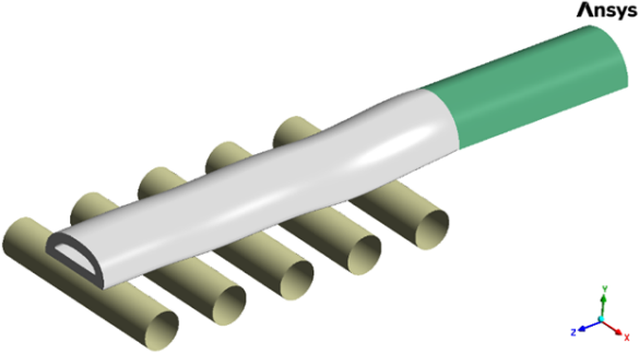
Figure 4.54: Simulation of the Extrusion of a Heavy Profile Assisted by Conveyor Rollers. The Fluid Flows From Right to Left. Important Components Are the Die Wall (Green), the Extrudate (Grey) and the Conveyor Rollers (Brown) depicts a typical extrusion line for the fabrication of a heavy D-shaped rubber fender, which includes a number of conveyor rollers. The processed material flows through the die (green) from right to left, while the extrudate with a D-shaped cross-section (grey) develops at the die outlet. The extrudate falls onto the conveyor rollers (brown) due to gravity along the-y direction, which rotate around their respective axes at a speed that suits the process requirements.
The calculating domain includes a portion of the die channel and an extrudate region. It is bounded by six boundaries, each of which has the following conditions. The fluid material enters the computational domain via the inlet, at the right extremity of the die, in the upper-right corner of the image. Inside the D-shaped die channel, it flows from right to left with appropriate boundary conditions along both the inner and outer walls. The free surface conditions apply on both the inner and outer bundaries of the extrudate as it is drawn downwards by gravity onto the conveyor rollers at the die exit. A take-up velocity compatible to the rotation velocity of the conveyor rollers is imposed at the calculation domain's exit. The current conveyor consists of five rollers that rotate at an angular velocity that matches the take-up velocity.
Figure 4.55: Cross Section of the Die Channel and Location of the Conveyor Rollers depicts a cross-section of the die channel as well as the location of the conveyor rollers beneath it. The shape resembles a D fender profile and is made out of a hollow half disk with a radius of 0.1 m and a wall thickness of 0.025 m. The box enclosing the entire computational domain (die channel and extrudate without rollers) measures 0.2x0.1x1.550 [m]. The die channel has a width of 0.2 m and a maximum height of 0.1 m. The conveyor rollers are situated 0.02 m below the die channel exit, as shown in Figure 4.55: Cross Section of the Die Channel and Location of the Conveyor Rollers. There are five cylindrical rollers in a horizontal sequence, separated by 0.2 m between two succeeding cylinder axis. The rollers can be defined one by one, or as a series; the latter way is preferred when the rollers are positioned at regular interval. Finally, the die and extrudate lengths are 0.5 and 1.05 m, respectively.
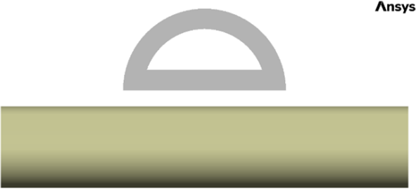
The fluid density and viscosity are 1200 kg/m3 and 105 Pa.s respectively. The inlet mass flow rate is 0.65 kg/s and a take-up velocity of 0.05 m/s is applied at the exit section, while each roller rotates with an angular velocity of 1 rad/s. Therefore, the tangential velocity matches the take-up velocity at the exit of the computational domain. The gravity (along the y-direction) has a value -9.81 m/s2. Vanishing velocity is assumed along the die wall. However, for the sake of convergence, this condition is replaced by a linear slipping law with a high coefficient and continuation, partial slipping is assumed on the conveyor rollers.
Although a simple rheology is selected for the fluid, the flow involves non-linearities and large element deformations as well. Hence, appropriate convergence strategies and continuation approach will be used. Default convergence strategy for moving boundaries, as well as an expression on the gravity and on the slipping coefficient defined on the die wall are applied.
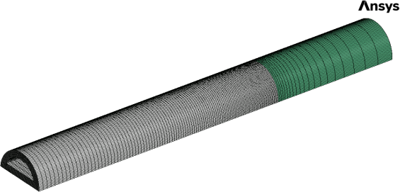
Figure 4.56: Finite Element Mesh shows a sketch of the presently selected mesh. It consists of around 75000 hexahedra elements with a mapped distribution. Relatively small elements are chosen all along the extrudate to properly represent any sagging deformations that may occur between two succeeding rollers. Smaller elements are also chosen around the die exit. The entry and exit cross sections each include approximately 580 quadrilateral pieces.
The following sections describe the setup and solution steps for this example:
To prepare for running this example:
Download the
d_fender.zipfile here .Unzip
d_fender.zipto your working directory.The file,
d_fender.poly, can be found in the folder.Use Fluent Launcher to start the Fluent Materials Processing workspace, with the Capability Level set to Enterprise.
Select an extrusion simulation template for this example. When you choose a template, the Fluent Materials Processing workspace generates a skeleton based on your selection, so you typically only need to fill up a few fields. Typically, fluid material data must be supplied. Cell zones must be created, boundary constraints provided, and a mesh deformation method (for extrudate section) specified. Before conducting the calculation, solver options must be selected.
![]() Setup → Simulation → Use
Template...
Setup → Simulation → Use
Template...
This displays the Simulation Template dialog box, where you can specify particular details for the type of simulation.
Set the Type to Extrusion.
Set the Goal to Predict extrudate shape.
Click Apply to close the dialog box. The workspace will set up the various requirements for the specified simulation type.
![]() Setup → General
Setup → General
This displays the Properties - General panel.
Set the Calculation Type to Continuation.
Enable the option.
Click the arrow to the right of Gy [m/s^2] and select .
Set Gy to -9.81 * time [m/s^2]. This outlines a gradual involvement of gravity, where time represents a pseudo-time.
Define the material properties for the fluid.
![]() Setup → Materials →
fluid
Setup → Materials →
fluid
Expand the Density Law in the properties view.
Set the Density to 1200 kg/m3.
Expand the Viscosity Law in the properties view.
Set the Viscosity to 100000 [Pa s].
Define the cell zone properties for the fluid-zone.
![]() Setup → Cell Zones →
fluid-zone
Setup → Cell Zones →
fluid-zone
Set the Zones to include die and extrudate.
Define the fluid boundary conditions.
Define fluid boundary conditions at the extrudate-exit.
Setup → Fluid Boundary
Conditions → extrudate-exitSet the Boundary Zone to exit.
Set Flow Specification to Take-up velocity.
Set Vx to 0.0 [m/s].
Set Vy to 0.0 [m/s].
Set Vz to 0.05 [m/s].
Define conditions for free-surface.
Setup → Fluid Boundary
Conditions → free-surfaceSet the Boundary Zone to outerfs.
Set the Fixed Part to outerwall (the attachment line of the free surface).
Define conditions at the inlet.
Setup → Fluid Boundary
Conditions → inletSet the Boundary Zone to inlet.
Set the Flow Specification to Mass flow.
Set the Mass Flow Rate to 0.65 kg/s.
Define conditions at the wall.
Setup → Fluid Boundary
Conditions → wallSet the Boundary Zone to innerwall and outerwall.
Set the Slip Specification to Partial slip.
Set the Slip Model to Navier law.
Click the arrow to the right of Friction Coefficient and select .
Set the Friction Coefficient to 1e8 * time Pa. This defines a progressive rise in friction, where time represents a pseudo-time.
Define a new fluid boundary condition.
Setup → Boundary Conditions
→ Fluid → New →
Free surfaceChange the Name to free-surface-2.
Set the Boundary Zone to innerfs.
Set the Fixed Part to innerwall (the attachment line of the free surface).
Define the guiding devices
Define a new guiding device.
Setup → Boundary Conditions
→ Guiding Device → New →
Roller ConveyorSet the Number of Rollers to 5.
Set the Radius to 0.05 [m].
Set Xo to -0.2 [m].
Set Yo to -0.07 [m].
Set Zo to 0.2 [m].
Set Xe to 0.2 [m].
Set Ye to -0.07 [m].
Set Ze to 0.2 [m].
Set Dx to 0.0 [m].
Set Dy to 0.0 [m].
Set Dz to 0.2 [m].
Set Omega to 1 [rad/s].
Set Free Surfaces to outerfs.
Set the Slipping Coefficient to 1000 [kg/(m^2 s)].
Set the Penalty Coefficient to 1.e7 [kg/(m^2 s^2)].
Click Display in order to see the roller conveyor
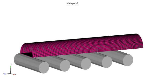
Define the conditions for the various mesh deformations in the simulation.
Define the mesh deformation conditions for the extrudate.
Setup → Mesh Deformations
→ extrudateSet the Zones to extrudate.
Set the Inlet Section to extrudate-die.
Set the Outlet Section to exit.
Define any particular solution-based settings in the simulation.
Define the derived quantities.
Solution → Derived Quantities Select any quantities that are of interest.
Define any calculation activities.
Solution → Calculation
Activities Set the Solver Type to AMF direct solver + secant.
For Convergence Strategies, select Free Surfaces and Moving Interfaces.
Run the calculations.
The setup is now ready and it can now be checked, and the calculation can start.
Solution → Run Calculation Click Check to perform a final check of the setup and the coherence of the data.
If there are no errors or warnings, click Calculate.
The calculation converges in seven steps and around forty minutes using the free surface convergence strategy and the continuation approach.
The first piece of relevant information is the overall pressure drop of about 350 bars that develops over the 0.5-m long die channel. This very high value is most likely due to the high and constant viscosity of the melt, as well as to the nearly sticking boundary conditions assumed on the die walls. Actual materials such as uncured rubber do exhibit shear-thinning as well as wall slippage. Also, a typical wall shear rate inside the die is of about 10 s -1 with -1 as an exponent. This originates from the relatively low velocity involved which is required by the large dimensions of the extruded profile. To examine the results, inspect the calculated fields on the boundary of the calculation domain, as well as in several cross-sections perpendicular to the main flow direction, defined with an interval of 0.125 m from the inlet (located at z = -0.5 m) to the domain exit (located at z = 1.05 m).
Figure 4.58: Velocity Magnitude on Extrudate and on Some Cutting Planes in the Die depicts the distributions of the fluid's velocity magnitude on the extrudate's outside border as well as the various cross sections defined within the die. The very low velocity of the fluid along the die walls can be identified since the walls are supposed to have almost zero velocity. You will also notice that the conveyor rollers drag the fluid, which is particularly obvious in sections of the free surface where the velocity magnitude is developed and equals the actual tangential velocity of 0.05 m/s at the rollers' surface.
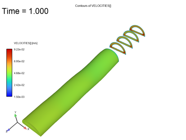
Figure 4.59: Velocity Distribution on All Cross-Sections shows the distributions of the fluid's velocity magnitude in all cross sections defined inside the die and extrudate. Figure 4.60: Velocity Vectors on All Cross Sections on All Cross-Sections shows the corresponding velocity vectors. Here you can observe how the extrudate shape evolves and eventually attains the velocity of the conveyor rollers. If the contact with the conveyor rollers had a zero-slipping coefficient (for example, full slipping), the extrudate shape would spread over a greater distance.
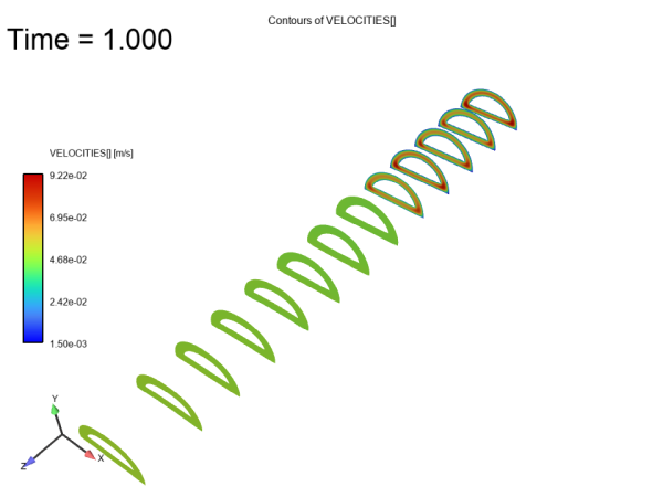
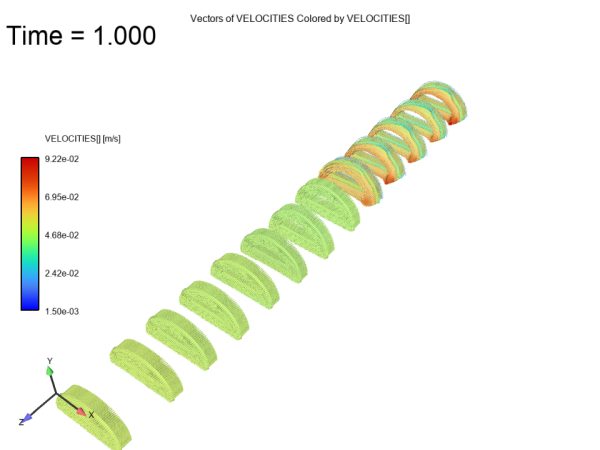
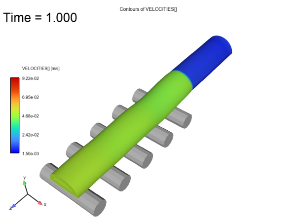
Start CFD-Post.
![]() Results
Results ![]() CFD-Post
CFD-Post
It is possible to display the final extrudate and the five rollers. Transparency of the extrudate allows to observe the contact between the outer free surface and conveyor rollers.
Figure 4.62: Final Shape and Position of the Extrudate With Respect to the Rollers Displayed in CFD-Post