You can use the following process to code a UDF and use it effectively in your Ansys Fluent model.
For more information, see the following sections:
- 8.1.1. Process Overview
- 8.1.2. Step 1: Define Your Problem
- 8.1.3. Step 2: Create a C Source File
- 8.1.4. Step 3: Start Ansys Fluent and Read (or Set Up) the Case File
- 8.1.5. Step 4: Interpret or Compile the Source File
- 8.1.6. Step 5: Hook the UDF to Ansys Fluent
- 8.1.7. Step 6: Run the Calculation
- 8.1.8. Step 7: Analyze the Numerical Solution and Compare to Expected Results
To begin the process, you’ll need to define the problem you want to solve using a UDF (Step 1). For example, suppose you want to use a UDF to define a custom boundary profile for your model. You will first need to define the set of mathematical equations that describes the profile.
Next you will need to translate the mathematical equation (conceptual
design) into a function written in the C programming language (Step
2). You can do this using any text editor. Save the file with a .c suffix (for example, udfexample.c) in your working folder. (See Appendix A: C Programming Basics for some basic information
on C programming.)
After you have written the C function, you are ready to start Ansys Fluent and read in (or set up) your case file (Step 3). You will then need to interpret or compile the source code, debug it (Step 4), and then hook the function to Ansys Fluent (Step 5). Finally you’ll run the calculation (Step 6), analyze the results from your simulation, and compare them to expected results (Step 7). You may loop through this entire process more than once, depending on the results of your analysis. Follow the step-by-step process in the sections below to see how this is done.
The first step in creating a UDF and using it in your Ansys Fluent model involves defining your model equation(s).
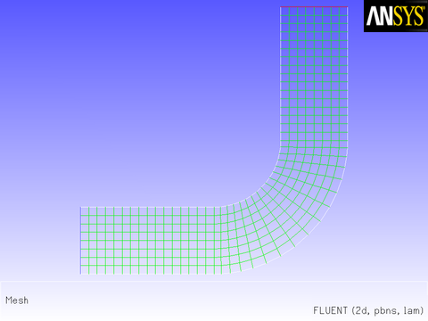
Consider the elbow duct illustrated in Figure 8.1: The Mesh for the Elbow Duct Example. The domain has a velocity inlet on the left side, and a pressure outlet at the top of the right side.
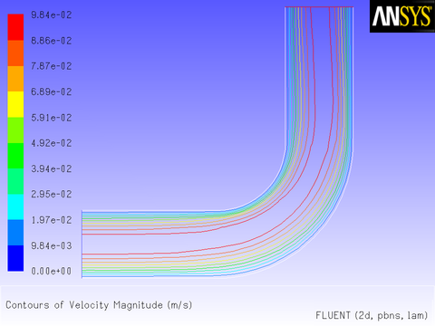
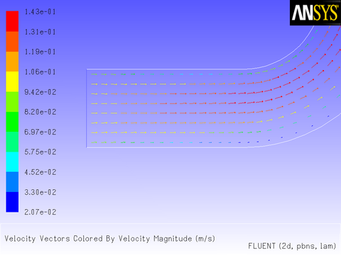
A flow field in which a constant x velocity is applied at the inlet will be compared with one where a parabolic x velocity profile is applied. The results of a constant velocity (of 0.1 m/s) at the inlet are shown in Figure 8.2: Velocity Magnitude Contours for a Constant Inlet x Velocity and Figure 8.3: Velocity Vectors for a Constant Inlet x Velocity.
Now suppose that you want to impose a non-uniform x velocity to the duct inlet, which has a parabolic shape. The velocity is 0 m/s at the walls of the inlet and 0.1 m/s at the center.
To solve this type of problem, you can write a custom profile UDF and apply it to your Ansys Fluent model.
Now that you have determined the shape of the velocity profile
that defines the UDF, you can use any text editor to create a file
containing C code that implements the function. Save the source code
file with a .c extension (for example, udfexample.c) in your working folder. The following UDF
source code listing contains only a single function. Your source file
can contain multiple concatenated functions. (Refer to Appendix A: C Programming Basics for basic information on
C programming.)
Below is an example of how the profile described in Step 1 can
be implemented in a UDF. The functionality of the UDF is designated
by the leading DEFINE macro. Here, the DEFINE_PROFILE macro is used to indicate to the solver
that the code that follows will provide profile information at boundaries.
Other DEFINE macros will be discussed later
in this manual. (See
DEFINE Macros for
details about DEFINE macro usage.)
/***********************************************************************
   udfexample.c
  UDF for specifying steady-state velocity profile boundary condition
 ************************************************************************/

 #include "udf.h"

 DEFINE_PROFILE(inlet_x_velocity, thread, position)
 {
    real x[ND_ND]; /* this will hold the position vector */
    real y, h;
    face_t f;
    h = 0.016; /* inlet height in m */
    begin_f_loop(f,thread)
    {
      F_CENTROID(x, f, thread);
      y = 2.*(x[1]-0.5*h)/h; /* non-dimensional y coordinate */
      F_PROFILE(f, thread, position) = 0.1*(1.0-y*y);
    }
    end_f_loop(f, thread)

 }
The first argument of the DEFINE_PROFILE macro, inlet_x_velocity, is the name of
the UDF that you supply. The name will appear in the boundary condition
dialog box after the function is interpreted or compiled, enabling
you to hook the function to your model. Note that the UDF name you
supply cannot contain a number as the first character. The equation
that is defined by the function will be applied to all cell faces
(identified by f in the face loop) on a given
boundary zone (identified by thread). The
thread is defined automatically when you hook the UDF to a particular
boundary in the Ansys Fluent GUI. The index is defined automatically through
the begin_f_loop utility. In this UDF, the begin_f_loop macro (Looping Macros) is used to loop through
all cell faces in the boundary zone. For each face, the coordinates
of the face centroid are accessed by F_CENTROID (Face Centroid (F_CENTROID)). The  coordinate
 y is used in the parabolic profile equation and the returned velocity
is assigned to the face through F_PROFILE. begin_f_loop and F_PROFILE (Set Boundary Condition Value (F_PROFILE)) are Ansys Fluent-supplied
macros. Refer to Additional Macros for Writing UDFs for
details on how to utilize predefined macros and functions supplied
by Ansys Fluent to access Ansys Fluent solver data and perform other tasks.
After you have created the source code for your UDF, you are ready to begin the problem setup in Ansys Fluent.
Start Ansys Fluent in Windows using Fluent Launcher with the following settings:
Specify the folder that contains your case, data, and UDF source files in the Working Directory field in the General Options tab.
If you plan to compile the UDF, make sure that the batch file for the UDF compilation environment settings is correctly specified in the Environment tab (see Compilers for further details).
Read (or set up) your case file.
You are now ready to interpret or compile the profile UDF (named
inlet_x_velocity) that you created in Step
2 and that is contained within the source file named udfexample.c. In general, you must compile your function
as a compiled UDF if the source code contains structured reference
calls or other elements of C that are not handled by the Ansys Fluent interpreter.
To determine whether you should compile or interpret your UDF, see
Differences Between Interpreted and Compiled UDFs.
Follow the procedure below to interpret your source file in Ansys Fluent. For more information on interpreting UDFs, see Interpreting UDFs.
Important: Note that this step does not apply to Windows parallel networks. See Interpreting a UDF Source File Using the Interpreted UDFs Dialog Box for details.
Open the Interpreted UDFs dialog box.
 Parameters & Customization → User Defined Functions
  Interpreted...
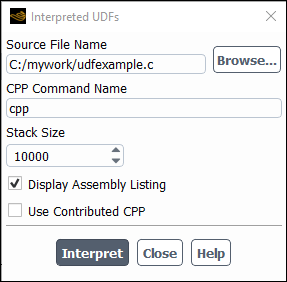
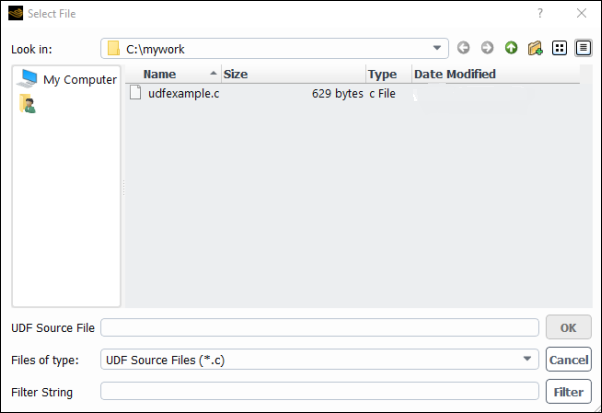
In the Interpreted UDFs dialog box, indicate the UDF source file you want to interpret by clicking the Browse... button. This will open the Select File dialog box (Figure 8.5: The Select File Dialog Box).
In the Select File dialog box, select the desired file (for example, udfexample.c) and click . The Select File dialog box will close and the complete path to the file you selected will appear in the Source File Name field in the Interpreted UDFs dialog box (Figure 8.4: The Interpreted UDFs Dialog Box).
In the Interpreted UDFs dialog box, specify the C preprocessor to be used in the CPP Command Name field. You can keep the default cpp or you can select Use Contributed CPP to use the preprocessor supplied by Ansys Fluent.
Keep the default Stack Size setting of
10000, unless the number of local variables in your function will cause the stack to overflow. In this case, set the Stack Size to a number that is greater than the number of local variables used.If you want a listing of assembly language code to appear in your console when the function interprets, enable the Display Assembly Listing option. This option will be saved in your case file, so that when you read the case in a subsequent Ansys Fluent session, the assembly code will be automatically displayed.
Click Interpret to interpret your UDF. If the Display Assembly Listing option was enabled, then the assembly code will appear in the console when the UDF is interpreted, as shown below.
inlet_x_velocity:
           .local.pointer thread (r0)
           .local.int position (r1)
    0      .local.end
    0      save
           .local.int x (r3)
    1      begin.data 8 bytes, 0 bytes initialized:
         .local.float y (r4)
    5      push.float 0
           .local.float h (r5)
    .      .
    .      .
    .      .
  142      pre.inc.int f (r6)
  144      pop.int
  145      b .L3 (28)
     .L2:
  147      restore
  148      restore
  149      ret.v
Important: Note that if your compilation is unsuccessful, then Ansys Fluent will report an error and you will need to debug your program. See Common Errors Made While Interpreting A Source File for details.
Click Close when the interpreter has finished.
Write the case file. The interpreted UDF will be saved with the case file so that the function will be automatically interpreted whenever the case is subsequently read.
You can compile your UDF using the text user interface (TUI) or the graphical user interface (GUI) in Ansys Fluent. The GUI option for compiling a source file on a Windows system is discussed below. For details about compiling on other platforms, using the TUI to compile your function, or for general questions about compiling UDFs in Ansys Fluent, see Compiling UDFs.
As mentioned previously, make sure that you have started Ansys Fluent in Windows using Fluent Launcher with the following settings:
Specify the folder that contains your case, data, and UDF source files in the Working Directory field in the General Options tab.
Make sure that the batch file for the UDF compilation environment settings is correctly specified in the Environment tab (see Compilers for further details).
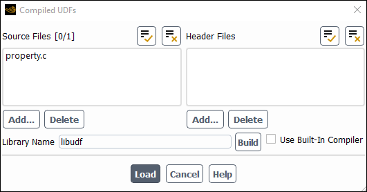
Open the Compiled UDFs dialog box (Figure 8.6: The Compiled UDFs Dialog Box).
Parameters & Customization → User Defined Functions Compiled...
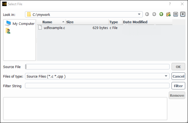
Click Add... under Source Files in the Compiled UDFs dialog box. This will open the Select File dialog box (Figure 8.7: The Select File Dialog Box).
In the Select File dialog box, select the file (for example,
udfexample.c) you want to compile. The complete path to the source file will then be displayed in the bottom list. Click . The Select File dialog box will close and the file you added will appear in the Source Files list in the Compiled UDFs dialog box.In a similar manner, select the Header Files that need to be included in the compilation.
In the Compiled UDFs dialog box, type the name of the shared library in the Library Name field (or leave the default name libudf).
If you installed a version of Microsoft Visual Studio or Clang on your machine that is older and not supported, then you should enable the Use Built-In Compiler option, in order to request the use of a built-in compiler (Clang) that is provided with the Fluent installation. If Fluent determines that you have not installed a compiler on your machine, the built-in compiler will be used automatically, whether or not you have enabled the Use Built-In Compiler option.
Click . This process will compile the code and will build a shared library in your working folder for the architecture you are running on.
As the compile/build process begins, a Question dialog box will appear, reminding you that the UDF source file must be in the folder that contains your case and data files (that is, your working folder). If you have an existing library folder (for example, libudf), then you will need to delete it prior to the build to ensure that the latest files are used. Click to close the dialog box and resume the compile/build process. The results of the build will be displayed in the console. You can view the compilation history in the
logfile that is saved in your working folder.Important: If the compile/build is unsuccessful, then Ansys Fluent will report an error and you will need to debug your program before continuing. See Common Errors When Building and Loading a UDF Library for a list of common errors.
Click Load to load the shared library into Ansys Fluent. The console will report that the library has been opened and the function (for example,
inlet_x_velocity) loaded.Opening library "E:\libudf"... Library "E:\libudf\win64\3d_host\libudf.dll" opened Opening library "E:\libudf"... Library "E:\libudf\win64\3d_node\libudf.dll" opened inlet_x_velocity Done.
See Compiling UDFs for more information on the compile/build process.
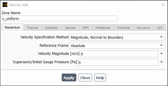
Now that you have interpreted or compiled your UDF following the methods outlined in Step 4, you are ready to hook the profile UDF in this sample problem to the Velocity Inlet boundary condition dialog box (see Hooking UDFs to Ansys Fluent for details on how to hook UDFs). First, click the Momentum tab in the Velocity Inlet dialog box (Figure 8.8: The Velocity Inlet Dialog Box) and then choose the name of the UDF that was given in our sample problem with udf preceding it (udf inlet_x_velocity) from the X-Velocity drop-down list. Click to accept the new boundary condition and close the dialog box. Your user profile will be used in the subsequent solution calculation.
![]() Setup →
Setup → ![]() Boundary
Conditions →
Boundary
Conditions → ![]() cold-inlet → Edit...
cold-inlet → Edit...
After initializing the solution, run the calculation.
![]() Solution → Run Calculation
Solution → Run Calculation ![]() Calculate
Calculate
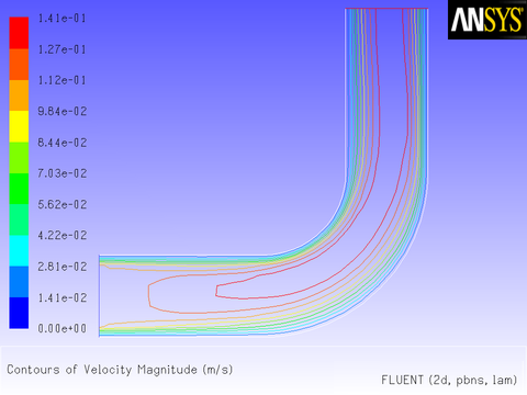
After the solution is run to convergence, obtain a revised velocity field. The velocity magnitude contours for the parabolic inlet x velocity are shown in Figure 8.9: Velocity Magnitude Contours for a Parabolic Inlet Velocity Profile, and can be compared to the results of a constant velocity of 0.1 m/s (Figure 8.2: Velocity Magnitude Contours for a Constant Inlet x Velocity). For the constant velocity condition, the velocity profile is seen to develop as the flow passes through the duct. The velocity field for the imposed parabolic profile, however, shows a maximum at the center of the inlet, which drops to zero at the walls.