


All properties for the Body Interactions folder are included in an Advanced category and define the global properties of the contact algorithm for the analysis. These properties are applied to all Body Interaction objects and to all frictional and frictionless manual contact regions.
This section includes descriptions of the following properties for the Body Interactions folder:
- 3.2.1.1. Contact Detection
- 3.2.1.2. Formulation
- 3.2.1.3. Sliding Contact
- 3.2.1.4. Manual Contact Treatment
- 3.2.1.5. Shell Thickness Factor and Nodal Shell Thickness
- 3.2.1.6. Body Self Contact
- 3.2.1.7. Element Self Contact
- 3.2.1.8. Tolerance
- 3.2.1.9. Pinball Factor
- 3.2.1.10. Time Step Safety Factor
- 3.2.1.11. Limiting Time Step Velocity
- 3.2.1.12. Edge on Edge Contact
The available choices are described below.
Trajectory
The trajectory of nodes and faces included in frictional or frictionless contact are tracked during the computation cycle. If the trajectory of a node and a face intersects during the cycle a contact event is detected.
The trajectory contact algorithm is the default and recommended option in most cases for contact in Explicit Dynamics analyses. Contacting nodes/faces can be initially separated or coincident at the start of the analysis. Trajectory based contact detection does not impose any constraint on the analysis time step and therefore often provides the most efficient solution.
Note that nodes which penetrate into another element at the start of the simulation will be ignored for the purposes of contact and thus should be avoided. To generate duplicate conforming nodes across a contact interface:
Use the multibody part option in DesignModeler and set Shared Topology to Imprint.
For meshing, use Contact Sizing, the Arbitrary match control or the Match mesh Where Possible option of the Patch Independent mesh method.
Proximity Based
The external faces, edges and nodes of a mesh are encapsulated by a contact detection zone. If during the analysis a node enters this detection zone, it will be repelled using a penalty-based force.
Note:
An additional constraint is applied to the analysis time step when this contact detection algorithm is selected. The time step is constrained such that a node cannot travel through a fraction of the contact detection zone size in one cycle. The fraction is defined by the Time Step Safety Factor described below. For analyses involving high velocities, the time step used in the analysis is often controlled by the contact algorithm.
The initial geometry/mesh must be defined such that there is a physical gap/separation of at least the contact detection zone size between nodes and faces in the model. The solver will give error messages if this criteria is not satisfied. This constraint means this option may not be practical for very complex assemblies.
Proximity Based Contact is not supported in 2D Explicit Dynamics analyses.
This property is available if Contact Detection is set to Trajectory.
The available choices are described below.
Penalty
If contact is detected, a local penalty force is calculated to push the node involved in the contact event back to the face. Equal and opposite forces are calculated on the nodes of the face in order to conserve linear and angular momentum.
Trajectory based penalty force, 
Proximity based penalty force, 
Where:
D is the depth of penetration
M is the effective mass of the node (N) and face (F)
Δt is the simulation time step
Note:
Kinetic energy is not necessarily conserved. You can track conservation of energy in contact using the Solution Information object, the Solution Output, or one of the energy summary result trackers.
The applied penalty force will push the nodes back towards the true contact position during the cycle. However, it will usually take several cycles to satisfy the contact condition.
When using trajectory contact with the penalty method, the calculated contact energy may have some inaccuracies that arise due to some assumptions made in the energy calculation. This may manifest in spurious-looking contact energy plots—for example, a negative contact energy when a positive contact energy is expected. These errors may be particularly prevalent if the simulation has:
A timestep that is changing over the period in which bodies are in contact
Contact interfaces that are sliding over one another
Erosion occurring at contact interfaces
In some situations, modifying the contact penalty factor using a command object may help to reduce the contact energy error.
Decomposition Response
All contacts that take place at the same point in time are first detected. The response of the system to these contact events is then calculated to conserve momentum and energy. During this process, forces are calculated to ensure that the resulting position of nodes and faces does not result in further penetration at that time point.
Note:
The decomposition response algorithm cannot be used in combination with bonded contact regions. The formulation will be automatically switch to penalty if bonded regions are present in the model.
The decomposition response algorithm is more impulsive (in a given cycle) than the penalty method. This can give rise to large hourglass energies and energy errors.
This option is available if Contact Detection is set to Trajectory.
When a contact event is detected part way through a cycle and the contact node has a tangential velocity relative to the face it has made contact with, the node needs to slide along the face for the remainder of the cycle. If the node should slide to the edge of the face before the end of the cycle, it is necessary to determine whether the node needs to begin to slide along an adjacent face. Two options described below are available for determining which (if any) face the node needs to slide to.
Discrete Surface
When a node slides to the edge of a face, the next face the node needs to slide on is determined using the contact detection algorithm. This option is the default and will provide the most time efficient solution. However, penetrations of nodes may be seen in situations where the faces that the nodes are sliding on are experiencing large deformations or rotations. When such penetrations occur, it is recommended the user switches to the Connected Surface option.
Connected Surface
When a node slides to the edge of a face, the next face the node needs to slide on is determined using the mesh connectivity.
This option is available if Sliding Contact is set to Connected Surface. It determines how combinations of manual contact regions and body interactions are handled in the Explicit Dynamics solver. Options are Pairwise and Lumped. When Lumped is selected, all regions that are scoped to a manual contact region are free to contact with each other. When Pairwise is selected, contact can only occur between a node and a face if the node appears in the contact scoping and the face in the target scoping of the same manual contact region. This is explained further in Manual Contact Regions in Explicit Dynamics Analyses.
These properties are available if the geometry includes one or more surface bodies and if Contact Detection is set to Trajectory.
The Shell Thickness Factor allows you to control the effective thickness of surface bodies used in the contact. The value of the factor must be between 0.0 and 1.0, and determines the amount of the shell thickness that is taken into account for the interaction distance. Typically, a value of 0.0 or 1.0 should be chosen.
Interaction in the solver is always taking place between a node and a face (contact surface). You can enable two (complementary) algorithms to take the shell thickness into account:
Shell thickness for the faces which will offset the faces
Shell thickness for the nodes which creates a "sphere" around the node
In order to use one or both of these thickness algorithms you can:
Set the shell thickness factor to a value other than zero to activate the shell thickness algorithm for the faces
Enable nodal shell thickness to activate the shell thickness algorithm for the nodes, in addition to shell thickness for the faces
Interaction Behavior with Shell Thickness
Setting the factor to a value other than zero means that the contact surface is positioned at (0.5 x shell thickness x factor) on both sides of the shell mid plane.
A factor of 0.0 means that the shell has no contact thickness and the contact surface is positioned at the shell mid plane. Note that with this setting the nodal shell thickness can not be activated separately.
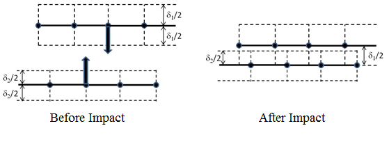
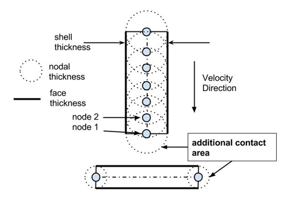
The contact area of a node depends on the setting for Nodal Shell Thickness. If it is set to No, the node is always located at the mid-surface of the shell (Situation I). If it is set to Yes, the node is located at a spherical distance of half the thickness away from the physical node location (Situation II).
Two shell parts with thickness δ1 and δ2 will not contact at a distance of (δ1/2 + δ2/2), but at a distance which is half of the largest shell thickness as is depicted below.
Note that for shell node on solid face impacts, the node will be able to get to within zero distance of the solid face; the thickness for the shell nodes will not be taken into account. The solid nodes will, however, find the shell faces at contact distance.
By enabling the nodal shell thickness, two shell parts will contact at a distance of (δ1/2 + δ2/2). From a physical point of view this is correct, as can be seen in the picture below.
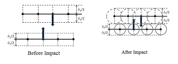
Note: Care should be taken for nodes that are on or close to a free edge of the shell surface because the node may find contact in an unexpected manner due to the spherical contact around these nodes. This is shown below in a 2D manner, where for example node 1 and 2 have an additional contact area which extends beyond the geometry.
When set to Program Controlled, the behavior of nodal shell thickness is determined by the Analysis Settings Preference Type.
When set to Yes, the contact detection algorithm will check for external nodes of a body contacting with faces of the same body in addition to other bodies. This is the most robust option since all possible external contacts should be detected.
When set to No, the contact detection algorithm will only check for external nodes of a body contacting with external faces of other bodies. This setting reduces the number of possible contact events and can therefore improve efficiency of the analysis. This option should not be used if a body is likely to fold onto itself during the analysis, as it would during plastic buckling for example.
When set to Program Controlled, the behavior of self contact is determined by the Analysis Settings Preference Type.
Presented below is an example of a model that includes self impact.
When set to Yes, automatic erosion (removal of elements) is enabled when an element deforms such that one of its nodes comes within a specified distance of one of its faces. In this situation, elements are removed before they become degenerated. Element self contact is very useful for impact penetration examples where removal of elements is essential to allow generation of a hole in a structure. Element removal through Element Self Contact is only activated when one of the erosion options under Erosion Controls is also set to Yes.
When set to Program Controlled, the behavior of self contact is determined by the Analysis Settings Preference Type.
This property is available if Contact Detection is set to Trajectory and Element Self Contact is set to Yes.
Tolerance defines the size of the detection zone for element self contact when the trajectory contact option is used (see Element Self Contact). The value input is a factor in the range 0.1 to 0.5. This factor is multiplied by the smallest characteristic dimension of the elements in the mesh to give a physical dimension. A setting of 0.5 effectively equates to 50% of the smallest element dimension in the model.
Note: The smaller the fraction the more accurate the solution.
This property is available if Contact Detection is set to Proximity Based.
The pinball factor defines the size of the detection zone for proximity based contact. The value input is a factor in the range 0.1 to 0.5. This factor is multiplied by the smallest characteristic dimension of the elements in the mesh to give a physical dimension. A setting of 0.5 effectively equates to 50% of the smallest element dimension in the model.
Note: The smaller the fraction, the more accurate the solution. The time step in the analysis could be reduced significantly if small values are used (see Time Step Safety Factor).
This property is available if Contact Detection is set to Proximity Based.
For proximity based contact, the time step used in the analysis is additionally constrained by contact such that in one cycle, a node in the model cannot travel more than the detection zone size, multiplied by a safety factor. The safety factor is defined with this property and the recommended default is 0.2. Increasing the factor may increase the time step and hence reduce runtimes, but may also lead to missed contacts. The maximum value you can specify is 0.5.
This property is available if Contact Detection is set to Proximity Based.
For proximity based contact, this setting limits the maximum velocity that will be used to compute the proximity based contact time step calculation.
This property is available if Contact Detection is set to Proximity Based.
By default, contact events in Explicit Dynamics are detected by nodes impacting faces. Use this option to extend the contact detection to include discrete edges impacting other edges in the model.
Note: This option is numerically intensive and can significantly increase runtimes. It is recommended that you compare results with and without edge contact to make sure this feature is required.
A model with edge on edge contact cannot be run in parallel.