


Material damage refers to the degradation of material stiffness due to microdefect initiation, propagation, and coalescence. Microdefect examples include voids and microcracks.
In the context of constitutive material models, microdefects are not explicitly represented as discrete geometrical features; rather, they are considered in a homogenized sense using the continuum damage-mechanics approach. Additional internal variables are introduced as a macroscopic measure of the distribution and the density of the microdefects.
The following material-damage topics are available:
In the simplest case of a uniform and isotropic distribution of microdefects in the
averaging domain, a scalar variable ranging from 0 (undamaged intact material) to 1 (full
degradation of the material) can be used. The so-called damage variable  relates the effective stress
  (acting on the material between the microdefects) to the nominal stress
 (acting on the homogenized material including the microdefects):

Assuming linear elastic behavior in the effective stress space, the nominal stress is rewritten as:

where  is the linear elastic material matrix, and
  is the total mechanical strain. In the equation above, the isotropic
degradation of the material stiffness by the damage parameter is directly expressed.
is the total mechanical strain. In the equation above, the isotropic
degradation of the material stiffness by the damage parameter is directly expressed.
For most materials, this simplified continuum damage formulation is insufficient. The damage effect might be anisotropic or the material behavior in the effective stress state might be nonlinear (such as plasticity or creep). Furthermore, the evolution of the damage parameters might be driven by different mechanisms (such as elasticity, plasticity, or creep).
Mechanical APDL provides multiple continuum damage models with varying levels of complexity. The following table summarizes the available damage models and their corresponding features:
| Continuum Damage Model | Damage Type | Damage Evolution |
|---|---|---|
| Fiber-reinforced material damage | Orthotropic | Elasticity-based |
| Elastic microplane damage | Anisotropic | Elasticity-based |
| Coupled microplane damage-plasticity | Anisotropic | Plasticity-based |
| Regularized generalized damage for fatigue and thermomechanical fatigue | Isotropic | Elasticity-/plasticity-/creep-based |
| Regularized anisotropic damage | Orthotropic | Plasticity-based |
| Ductile damage | Isotropic | Plasticity-based |
Damage usually results in a softening of the material. As damage develops, stress decreases with increasing strain. By modeling the material as a strain-softening continuum, this effect is explicitly considered within the stress-strain relationship of the constitutive model. (For example, the evolution of the damage parameter is expressed in terms of an equivalent strain measure.)
An effect related to material softening is strain-localization. If in a finite element model an element begins to soften, the neighboring elements are usually unloaded (decreasing strain), and damage and strain concentrate (localize) within a single layer of elements. During mesh refinement, the size of this critical region decreases, and the corresponding strains increase. In standard local continuum damage models with no regularization, this effect causes a pathological sensitivity of the results with respect to the element size. Furthermore, the solution might become unstable.
Mechanical APDL applies the following regularization methods to overcome such issues:
This table summarizes the regularization methods applied in the individual damage models:
| Continuum Damage Model | Regularization Method |
|---|---|
| Fiber-reinforced material damage | |
| Elastic microplane damage | |
| Coupled microplane damage-plasticity | |
| Regularized generalized damage for fatigue and thermomechanical fatigue | |
| Regularized anisotropic damage | |
| Ductile damage |
This regularization method is based on the crack band theory originally proposed by Bazant and Oh [5] for smeared crack models of concrete.
At element level, a characteristic element length  is introduced, and the stress-strain relationship is adjusted depending on
this quantity. It is assumed that the characteristic element length (calculated internally based
on the actual element geometry) represents the width of the localization zone.
is introduced, and the stress-strain relationship is adjusted depending on
this quantity. It is assumed that the characteristic element length (calculated internally based
on the actual element geometry) represents the width of the localization zone.
In Mechanical APDL damage models, the damage-evolution law is modified. Instead of directly using
an equivalent strain such as quantity  , the damage parameter is defined as a function of a corresponding equivalent
relative displacement
, the damage parameter is defined as a function of a corresponding equivalent
relative displacement  . As a result, the spurious mesh dependency of the damage variable itself and
the related nominal stresses is significantly reduced.
. As a result, the spurious mesh dependency of the damage variable itself and
the related nominal stresses is significantly reduced.
This approach does not limit the size of the localization zone; rather, localization of strains at element level is a fundamental assumption of this method. Consequently, the size of the localization zone decreases on mesh refinement. The corresponding strains remain mesh-dependent within the damaged region. This method nevertheless preserves the correct amount of energy dissipated during the damage process. Important results (such as damage, stresses, or deformation) are objective with respect to mesh refinement.
For more information about how the characteristic element length is calculated, see:
Use viscous regularization to overcome stability issues during the solution of a damaged structure. A rate effect is introduced in the damage formulation:

where:
 = rate-independent damage variable defined by the standard damage-evolution
law = rate-independent damage variable defined by the standard damage-evolution
law |
 = corresponding rate-dependent viscous damage variable = corresponding rate-dependent viscous damage variable |
 = a characteristic viscous relaxation time = a characteristic viscous relaxation time |
The nominal stress is redefined in terms of the viscous damage variable:

This modification results in a general rate-dependency of the damage evolution. If the viscous effect is introduced for stabilization only, the characteristic viscous relaxation time must be significantly smaller than the time step of the load step:

In the context of cyclic loading where each load cycle comprises individual load segments,
 is the time step of such a segment. If this condition is not satisfied, a
spurious rate-dependency of the results occurs.
is the time step of such a segment. If this condition is not satisfied, a
spurious rate-dependency of the results occurs.
The viscous regularization is an optional feature, applied in addition to the crack-band regularization.
For more information about viscous regularization, see:
Singularities caused by local strain-softening material models often lead to ill-posed differential equations, unconverged numerical results, and mesh sensitivity. The problem can be mitigated via implicit gradient regularization, a class of nonlocal methods, where local variables are enhanced by considering their nonlocal counterparts as extra degrees of freedom governed by Helmholtz-type equations.
The governing equations are therefore given by the linear momentum-balance equation and
modified Helmholtz equations describing the nonlocal equivalent strain field  :
:
(4–93) |
where:
 = Cauchy stress tensor = Cauchy stress tensor |
 = body force = body force |
 = nonlocal variable = nonlocal variable |
 = local variable to be enhanced = local variable to be enhanced |
 = length-scale parameter = length-scale parameter |
 = unit normal vector to the outer boundary of the nonlocal field = unit normal vector to the outer boundary of the nonlocal field |
The gradient regularization enhances the continuum damage model, where  is the local variable to be enhanced, and
  is the nonlocal counterpart.
The length-scale parameter  controls the range of nonlocal interaction. For hints about identifying the
length-scale parameter, see Identifying the Nonlocal Interaction-Range Parameter c.
controls the range of nonlocal interaction. For hints about identifying the
length-scale parameter, see Identifying the Nonlocal Interaction-Range Parameter c.
With the homogeneous Neumann boundary conditions  , no explicit definition of boundary conditions for the extra degrees of
freedom is required.
, no explicit definition of boundary conditions for the extra degrees of
freedom is required.
In contrast to the crack-band regularization approach, this method introduces a
localization limiter, represented by the length-scale parameter  . Consequently, the size of the damage zone and the corresponding strains
become insensitive to the mesh size.
. Consequently, the size of the damage zone and the corresponding strains
become insensitive to the mesh size.
The implicit gradient regularization method introduces additional degrees of freedom for the nonlocal variables. The following coupled pore-pressure-thermal mechanical solid elements support this regularization method: CPT212, CPT213, CPT215, CPT216, and CPT217. The nonlocal degree of freedom is activated via KEYOPT(18).
For more information, see:
You can control the Newton-Raphson out-of-balance loads caused by the extra degrees of freedom by setting the reference value and tolerance for the gradient field residual (CNVTOL,GFRS). You can also control the displacement convergence related to the extra degrees of freedom (CNVTOL,GFV).
Example 4.46: Setting the Gradient Field Residual and Displacement Tolerances
CNVTOL,GFRS,1e-7,.001
CNVTOL,GFV,1e-4,1e-5
Automatic time-stepping uses an internal heuristic to adjust the time increment. You can set an additional time-stepping control (CUTCONTROL,DMGLIMIT) to limit the maximum allowable damage increment in a time step.
The following topics about the fiber-reinforced damage option are available:
This data table defines the criteria type for determining the onset of material damage under loading.
Specify the TBOPT value on the TB,DMGI
command to correspond to failure criteria (TBOPT = 1 or FCRT).
The following table shows the coefficient values addressed for the
TBOPT values:
| Constants |
TBOPT = 1 or FCRT |
|---|---|
NPTS = 4 | |
| C1 | Failure criteria type for the tensile fiber failure mode[a] |
| C2 | Failure criteria type for the compressive fiber failure mode[a] |
| C3 | Failure criteria type for the tensile matrix failure mode[a] |
| C4 | Failure criteria type for the compressive matrix failure mode[a] |
[a] Valid failure criteria types:
| 1 -- Maximum strain |
| 2 -- Maximum stress |
| 3 -- Puck |
| 4 -- Hashin |
| 5 -- LaRc03 |
| 6 -- LaRc04 |
| 11 -- User-defined #1 |
| . . . |
| 19 -- User-defined #9 |
To complete the material damage definition, it is also necessary to specify a compatible material damage-evolution law (TB,DMGE). Without a damage-evolution law, the damage-initiation criteria have no effect on the material. The following table summarizes the compatible damage-evolution laws with specific damage-initiation criteria:
This data table defines the material damage-evolution law (or the way a material degrades) following the initiation of damage (TB,DMGE).
Specify the TBOPT value on the TB,DMGE
command to correspond to the instant stiffness reduction (TBOPT = 1
or MPDG).
The following table shows the coefficient values addressed for the available
TBOPT values:
| Constants |
TBOPT = 1 or MPDG |
|---|---|
NPTS = 4 | |
| C1 | Tensile fiber stiffness reduction[a] |
| C2 | Compressive fiber stiffness reduction[a] |
| C3 | Tensile matrix stiffness reduction[a] |
| C4 | Compressive matrix stiffness reduction[a] |
[a] Valid values are >=0 and <=1, where 0 = no reduction in material stiffness in the affected mode after damage initiation, and 1 = complete stiffness loss in the affected mode.
| Constants |
TBOPT = 2 or CDM |
|---|---|
NPTS = 8 | |
| C1 | Energy dissipated per unit area from tensile fiber damage |
| C2 | Viscous damping coefficient for tensile fiber damage |
| C3 | Energy dissipated per unit area from compressive fiber damage |
| C4 | Viscous damping coefficient for compressive fiber damage |
| C5 | Energy dissipated per unit area from tensile matrix damage |
| C6 | Viscous damping coefficient for tensile matrix damage |
| C7 | Energy dissipated per unit area from compressive matrix damage |
| C8 | Viscous damping coefficient for compressive matrix damage |
Table 4.38: Energies Dissipated per Unit Area
|
Energies dissipated per unit area Gc are specified individually for all damage modes (fiber tension, fiber compression, matrix tension, and matrix compression). For a specific damage mode, Gc is given by: For complex stress state, the equivalent stresses and strains are calculated based on Hashin failure criteria. 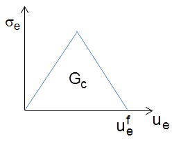
|


To complete the material damage definition, it is also necessary to specify a compatible material damage-initiation criterion (TB,DMGI). Without a damage-initiation criterion, the damage-evolution law has no effect on the material. The following table summarizes the compatible damage-initiation criteria with specific damage-evolution laws:
TB,DGME,,,,TBOPT option | Compatible TB,DMGI Input C1, C2, C3, C4 | |
TBOPT value | C1, C2, C3, C4 | |
| 1 or MPDG | 1 | 1, 2, ..., 19 |
| 2 or CDM | 1 | 4 (Hashin failure criteria only) |
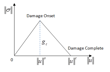
Use the progressive damage model (TB,DMGE) to predict post-damage degradation of brittle anisotropic materials, typically in fiber-reinforced composites. The undamaged material must be linearly elastic. The onset of damage is determined via failure criteria (TB,DMGI). For more information, see Failure Criteria in the Mechanical APDL Theory Reference.
Following the onset of damage, material stiffness reduction occurs immediately. The constitutive relationship for a damage material is given as:

For a general orthotropic material, the damaged elastic matrix is defined as:

For a transversely isotropic material with plane stress state, primarily adopted for thin fiber-reinforced composite structures, the damaged elastic matrix can be expressed as:

Four damage modes (fiber tension [rupture], fiber compression [kinking], matrix tension [cracking], and matrix compression [crushing]) are accounted for. Four damage variables (one for each mode) are used to measure damage. The damage variables for calculating the damaged elasticity matrix are determined as follows:

When a damage mode is initiated, the damage progresses immediately, indicated by the increasing damage variable for the mode.
Two damage-evolution methods are available:
Material property degradation method (TB,DMGE,,,,MPDG)
The material stiffness is instantly reduced based on the damage variables, explicitly specified via the TB,DMGE command. Any physical failure criteria can be used to detect the onset of the damage.
Continuum damage mechanics method (TB,DMGE,,,,CDM)
Damage variables increase gradually based on the energy amounts dissipated for the various damage modes. To achieve an objective response, the dissipated energy for each damage mode is regularized as follows:
The characteristic length Le is calculated from the element area A via the following expressions:
With this characteristic length, the constitutive relation is converted from stress-strain to stress-displacement relation. The damage-evolution function is derived from Hashin failure criteria; therefore, only Hashin failure criteria are allowed via TB,DMGI for detecting damage onset. For a plane stress state, the equivalent displacements
 and equivalent stresses
  are given below for all damage modes.


Four damage modes can be accounted for via the progressive damage model:
| Fiber Tension Damage Mode |  To ensure the continuity near the free fiber stress state
 |
| Fiber Compression Damage Mode |  |
| Matrix Tension Damage Mode |  |
| Matrix Compression Damage Mode |  |

In expressions above,  is the McCauley operator, defined as
  .
.
The damage variable d for a given mode is given as follows:

This section describes a material-agnostic material-damage law applicable for fatigue analysis (coupled mechanical-damage) and thermomechanical fatigue analysis (coupled thermal-mechanical-damage):
- 4.25.4.1. Understanding Generalized Damage
- 4.25.4.2. Material Mechanical Response
- 4.25.4.3. Gradient Regularization and Local Internal Variable
- 4.25.4.4. Degradation of Stress and Material Tangent
- 4.25.4.5. Thermal Evolution and Dissipation
- 4.25.4.6. Defining the Generalized Damage Model
- 4.25.4.7. Generalized Damage Output
Structural components are often exposed to significant cyclic thermal loading and complex force loading simultaneously, leading to fatigue failure due to damage initiation and propagation through the component materials. Following the onset of damage, an ill-posed partial differential equation system is a common problem in strain-softening and damage materials. The implicit gradient-regularized approach addresses the issue.
Because a wide range of material types are used in various engineering applications, the material-damage law makes no specific assumptions about any given material law. Instead, a general framework ensures that the stresses, material tangent, and other solution-history variables are determined in a consistent manner based on general material inelastic quantities.
Damage initiation and evolution are driven by the accumulation of inelasticity. A regularized fatigue variable is determined and then used to apply the influence of damage to the stress, material tangent, and inelastic dissipation. The thermal governing law is derived to account for material dissipation due to inelastic characteristics. The result is a multi-field problem consisting of the strain field, the nonlocal variable, and the temperature, leading to a fully coupled system.
The generalized-damage option uses the following assumptions for the material model:
The model considers additive decomposition of inelastic strain
 . For a plasticity-only material model
  and
and  , for a creep-only material model
  and
and  , and for a combined creep-plasticity material model
  and
and  .
.The inelastic material is defined in effective stress space (where the inelastic part is not coupled to damage). The material algorithm solving the inelastic part is decoupled from the damage evolution, enabling standard inelastic material models to calculate the effective stress.
Small-strain inelasticity:
Additive split of total strain into elastic, inelastic, and thermal strains:

The effective stress is a function of elastic strains (for example, for linear elasticity):

The inelasticity model provides the general material inelastic quantities used to develop the generalized damage framework:
Effective stress

Inelastic strain increment

Tangent matrix

It is further assumed that the damage is isotropic in nature. After the damage is
calculated in the manner shown in Degradation of Stress and Material Tangent, the effective stress
 can be degraded to obtain the nominal stress
  :
:

The generalized damage model supports the following materials:
The governing equation for the nonlocal equivalent strain field is shown in Implicit Gradient Regularization.
The local internal variable representing the local deformation is:[1]
 , where
where:
 = normalization constant of the equivalent inelastic strain rate = normalization constant of the equivalent inelastic strain rate |
 = power index representing the time dependence of the lifetime fatigue
behavior: = power index representing the time dependence of the lifetime fatigue
behavior: |
leads to rate-independent behavior
leads to a fully time-dependent lifetime behavior[5]
 = normalization constant of the von Mises equivalent effective (undamaged)
stress = normalization constant of the von Mises equivalent effective (undamaged)
stress  (defined as = (defined as =  , where , where  is the effective deviatoric stress) is the effective deviatoric stress) |
 = stress-dependency exponent = stress-dependency exponent |
 = magnitude of the inelastic strain rate increment = magnitude of the inelastic strain rate increment  , where the magnitude of the inelastic strain increment is defined as , where the magnitude of the inelastic strain increment is defined as
 with the assumption of additive decomposition of the inelastic strain with the assumption of additive decomposition of the inelastic strain
 . . |
The damage exponential function calculates the damage  when the nonlocal variable
  reaches the threshold
  :
:

where the damage rate coefficient  describes the rate at which the damage grows.
  is the Macauley bracket.
The governing equation for heat-transfer from Equation 4–92. The equation is rewritten to include the inelastic dissipation source:

where the inelastic dissipation rate  is a function of the nominal stress
  and is calculated as
  (where
  is the inelastic-dissipation-rate fraction coefficient).
For simplicity, other source and body-force terms have not been included here in the heat-transfer equation.
The following coupled pore-pressure-thermal mechanical solid elements support the generalized damage model: CPT212, CPT213, CPT215, CPT216, and CPT217.
For nonlocal damage, set KEYOPT(18) = 1 to activate the required extra degree of freedom (GFV1). The extra degree of freedom has no boundary-condition input.
A fine mesh is recommended, particularly at probable damage-prone regions. To observe
mesh-independent results, the mesh size may need to be less than half the square root of the
length-scale parameter  .[2]
.[2]
Define the inelastic material (TB). For example:
Define the damage parameters (TB,CDM,,,,GDMG), then specify the constants (TBDATA) for the CDM material data table:
| Constant | Meaning | Property | Unit | Range |
|---|---|---|---|---|
| C1 |  | Nonlocal parameter threshold | --- |  |
| C2 |  | Damage rate coefficient | --- |  |
| C3 |  | Stress dependency exponent | --- |  |
| C4 |  | Power index representing the time dependence of the lifetime fatigue behavior | --- |  |
| C5 |  | Normalization constant of the equivalent inelastic strain rate | Time-1 |  |
| C6 |  | Normalization constant of the equivalent effective stress | Force/Length2 |  |
| C7 |  | Length-scale parameter | Length2 |  |
Define Thermal Properties (if Needed)
The damage model is valid without the temperature degree of freedom active. If you wish to apply the effect of thermal evolution, activate the required extra degree of freedom (TEMP) via KEYOPT(11) = 1 and define the heat-transfer properties.
Optionally, define the inelastic dissipation rate fraction coefficient. If not explicitly defined, the default coefficient is 1. To change it, specify the new coefficient (TB,THERM,,,,DISS), then specify the constant (TBDATA) for the THERM material data table:
| Constant | Meaning | Property | Unit | Range |
|---|---|---|---|---|
| C1 |  | Inelastic dissipation rate fraction coefficient | --- |  Default: Default:  |
Example 4.48: Defining a Generalized Damage Model
/prep7
!Define element
ET,1,215
KEYO,1,18,1  ! nonlocal dof
KEYO,1,11,1  ! thermal dof

! parameters
rh=7860                  ! material density
cc=5.02e-4               ! heat capacity
k0=50                    ! thermal conductivity
alpha=10.8e-6            ! thermal expansion
temp_0=20.0              ! reference temperature

Em=2.35e5
nu=0.3
! Kinematic hardening
s0=400
gam1=2e2
gam2=1e2
Ck1=10
Ck2=5
Kr=1200
nn=1.5
br=6
Qr=1100

! Damage profile
c_eta=2.6
eta_cr=0
zz=0.06
! Fatigue damage
m0=1.0
n0=0.008
p0=0.6
a0=1.15e5

tb,elas,1
tbdata,1,Em,nu

tb,dens,1
tbdata,1,rh

tb,cte,1
tbdata,1,alpha

tref,temp_0

tb,therm,1,,,spht
tbdata,1,cc

tb,therm,1
tbdata,1,k0

tb,cdm,1,,,gdmg
tbdata,1,eta_cr,zz,m0,n0,p0,a0
tbdata,7,c_eta

TB,CHAB,1
TBDATA,1,s0,Ck1,gam1,Ck2,gam2

TB,RATE,1,,,EVH
TBDATA,1,s0,0,Qr,br,1/nn,Kr


This section describes a constitutive law for composite material with an anisotropic damage response at small deformations:
- 4.25.5.1.1. Understanding Regularized Anisotropic Damage
- 4.25.5.1.2. Gradient Regularization and Local Equivalent Strains
- 4.25.5.1.3. Mechanical Response of the Composite Material
- 4.25.5.1.4. Anisotropic Degradation of Stress and Material Tangent
- 4.25.5.1.5. Fiber and Damage Orientation
- 4.25.5.1.6. Defining the Anisotropic Damage Model
- 4.25.5.1.7. Anisotropic Damage Output
The regularized anisotropic damage option assumes a directionally-dependent elastic material. Stress and tangent quantities are consistently derived by applying a variational principle to the Helmholtz energy-density function.[2] Damage is accounted for by anisotropically degrading the components of the effective stress and material tangent. The model uses an implicit gradient regularization scheme, defined via a nonlocal field, that adds three extra degrees of freedom per node.
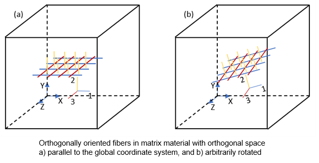
The fibers are assumed to be oriented along the axes of an orthogonal space. The orthogonal space, for both the anisotropic mechanical response and the anisotropic damage evolution, is assumed to be the same.
The governing equation for the nonlocal equivalent strain field from Equation 4–93 is rewritten to include an index
 . The index corresponds to the element coordinate system axes x, y, and z,
respectively, enabling parameter definition in the three orthogonal directions and resulting in
the anisotropic damage evolution:
. The index corresponds to the element coordinate system axes x, y, and z,
respectively, enabling parameter definition in the three orthogonal directions and resulting in
the anisotropic damage evolution:

where:
 = nonlocal variables = nonlocal variables |
 = local equivalent strains = local equivalent strains |
 = length-scale parameters = length-scale parameters |
The equivalent strain, representing the local deformation, is:

where the second invariant  is defined as:

and:
 = Poisson’s ratio of the matrix material = Poisson’s ratio of the matrix material |
 = first invariant of the small strain tensor = first invariant of the small strain tensor |
 = material parameter representing the ratio between the compressive strength = material parameter representing the ratio between the compressive strength
 and the tensile strength (that is, and the tensile strength (that is,  ) ) |
The value of  enables the model to account for the split in tension and compression damage
in the elastic domain.
enables the model to account for the split in tension and compression damage
in the elastic domain.
For the special case of  , the equivalent strain reduces to the standard von Mises definition
 .
.
A general anisotropic elastic model is used. The strain-energy density function is:

The strain energy density function has two components, both of which exhibit their own constitutive behavior:
Matrix (or bulk) material
Fiber reinforcement
The matrix material exhibits isotropic behavior, governed by the elastic parameters, bulk
modulus of elasticity  and bulk Poisson’s ratio
  .
.
The fiber parameters  ,
,  , and
, and  are direction-dependent with
  , corresponding respectively to the element coordinate system axes x, y,
z.
, corresponding respectively to the element coordinate system axes x, y,
z.
 is the fiber volume fraction,
  is the fiber modulus of elasticity, and
  is the fiber Poisson’s ratio.
 and
and  are the fourth and fifth invariants of the strain tensor, defined as

for  .
.
 is a unit vector representing the directions of the fiber orthogonal
space.
is a unit vector representing the directions of the fiber orthogonal
space.
The constitutive equations of the fiber reinforcings dictate that each fiber contributes
to the stiffness of the material in the spatial direction of its orientation only. The fibers
do not contribute to the material stiffness in directions other than their own spatial
direction of orientation. Also, shear effects between fibers  and
and  are not considered, simplifying the model (as the invariants of shear effects
 are ignored).
The overall anisotropic response is a consequence of the matrix material and fiber properties simultaneously.
The consistent material tangent  can be derived in the undamaged state:

where  and
and  are the second- and fourth-order identity tensors, respectively. The notation
 is defined in index form as:

The undamaged stress can be calculated as  .
.
The nominal stress  takes into account the effect of damage and is obtained by considering the
fourth-order damage tensor:
takes into account the effect of damage and is obtained by considering the
fourth-order damage tensor:

The fourth-order damage tensor is major symmetric and is expressed as:

The second-order tensor  reads:

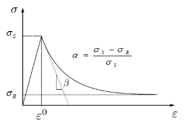
 is the softening function representing the damage components along the three
orthogonal directions. The softening function describes the material gradually losing stiffness
to damage. The softening function is defined by the exponential function:
is the softening function representing the damage components along the three
orthogonal directions. The softening function describes the material gradually losing stiffness
to damage. The softening function is defined by the exponential function:

where:
 = material parameters = material parameters |
 = equivalent strain thresholds = equivalent strain thresholds |
 = internal variables that preserve the history of the maximum values of the
corresponding nonlocal variables. = internal variables that preserve the history of the maximum values of the
corresponding nonlocal variables. |
The program uses the maximum values of the nonlocal variables  to prevent healing effects, as the damage evolution is irreversible.
 is therefore obtained as:

The influence of the softening parameters can be observed in a typical stress-strain response where  controls the slope following damage initiation and
  controls the residual stress following damage.
The fibers are assumed to be oriented in an orthogonal space. The damage evolution is
assumed to be oriented in the same orthogonal space as that of the fibers. Both the fiber and
damage parameters are indicated via indices  , where
  corresponds to the element coordinate system axes x, y, z,
respectively.
corresponds to the element coordinate system axes x, y, z,
respectively.
The initial fiber and damage orthogonal space is parallel to the element coordinate system. By default, the element coordinate system is parallel to the global coordinate system. Therefore, if an analysis requires an orientation of the fiber and damage that is not parallel to that of the global coordinate system, the element coordinate system must be rotated appropriately.
Example 4.49: Defining a Rotated Element Coordinate System
Issue these commands to define an element coordinate system rotated -45 degrees about the global Z axis:
LOCAL, 11, 0, 0, 0, 0, -45, 0, 0
ESYS,11
The following coupled pore-pressure-thermal mechanical solid elements support the anisotropic damage model: CPT212, CPT213, CPT215, CPT216, and CPT217.
To activate the required extra degrees of freedom (GFV1, GFV2, GFV3), set KEYOPT(18) = 3. The extra degrees of freedom have no boundary-condition input.
For 2D analysis (CPT212, CPT213), if out-of-plane damage is not of interest, set KEYOPT(18) = 2 to add two extra degrees of freedom at each corner node.
A fine mesh is recommended, particularly at probable damage-prone regions. To observe
mesh-independent results, the mesh size may need to be less than half the square root of the
length-scale parameter  .[3]
.[3]
Define the matrix elastic parameters (TB,ELAS).
Define the fiber parameters (TB,ELAS,,,,FIB1, TB,ELAS,,,,FIB2, and TB,ELAS,,,,FIB3) corresponding to the fiber directions along the element coordinate system x, y, z, respectively. If fibers are not desired in a given direction, the corresponding fiber parameter definition is not required for that direction. (For example, if fibers are desired only in direction 2, issue TB,ELAS,,,,FIB2 only.)
Specify the constants (TBDATA) for the ELAS material data table:
| Constant | Meaning | Property | Unit | Range |
|---|---|---|---|---|
| C1 |  | Fiber volume fraction | --- |  |
| C2 |  | Fiber elastic modulus | Force/Length2 |  |
| C3 |  | Fiber Poisson’s ratio | --- |  |
Define the damage parameters via TB,CDM,,,,FIB1, TB,CDM,,,,FIB2, and TB,CDM,,,,FIB3 corresponding to the damage directions along the element coordinate system x, y, z, respectively. If damage is not desired in a given direction, the corresponding damage parameter definition is not required for that direction. (For example, if damage is desired only in direction 2, issue TB,CDM,,,,FIB2 only.)
Specify the constants (TBDATA) for the CDM material data table:
| Constant | Meaning | Property | Unit | Range |
|---|---|---|---|---|
| C1 |  | Strength ratio | --- |  |
| C2 |  | Equivalent strain threshold | --- |  |
| C3 |  | Stress softening ratio parameter | --- |  |
| C4 |  | Stress softening slope parameter | --- |  |
| C5 |  | Length scale parameter | Length2 |  |
Example 4.50: Defining an Anisotropic Damage Model
/prep7
!Define element
ET,1,215
KEYO,1,18,3  ! Activate extra degrees of freedom

! Parameter values
cc1=5
cc2=5
cc3=5
EE0=21
nu0=0.18
ff1=0.103
EE1=190
nu1=0.18
ff2=0.0536
EE2=80
nu2=0.18
ff3=0
EE3=0
nu3=0
eps1=1.2*1.3e-4
eps2=1.2*1e-4
eps3=1.2*0.9e-4
alpha1=0.96
alpha2=0.96
alpha3=0.96
beta1=410
beta2=520
beta3=460
kk1=20
kk2=20
kk3=20

! Define matrix elastic properties of material
TB,ELAS,1
TBDATA,1,EE0,nu0

! Define fiber elastic properties
TB,ELAS,1,,,FIB1
TBDATA,1,ff1, EE1, nu1
TB,ELAS,1,,,FIB2
TBDATA,1,ff2, EE2, nu2
TB,ELAS,1,,,FIB3
TBDATA,1,ff3, EE3, nu3

! Define damage properties
TB,CDM,1,,,FIB1
TBDATA,1,kk1,eps1,alpha1,beta1,cc1
TB,CDM,1,,,FIB2
TBDATA,1,kk2,eps2,alpha2,beta2,cc2
TB,CDM,1,,,FIB3
TBDATA,1,kk3,eps3,alpha3,beta3,cc3

The ductile-damage option combines isotropic damage and small strain plasticity. The plastic part of the model is defined in the effective stress space:

where:
 = the total mechanical strain = the total mechanical strain |
 = plastic strain = plastic strain |
 = linear elastic material tensor = linear elastic material tensor |
The following plasticity models are supported:
von Mises Plasticity:
Bilinear isotropic hardening (TB,PLAS,,,,BISO)
Multilinear isotropic hardening (TB,PLAS,,,,MISO)
Nonlinear isotropic hardening (TB,NLISO)
Bilinear kinematic hardening (TB,PLAS,,,,BKIN)
Multilinear kinematic hardening (TB,PLAS,,,,KINH)
Chaboche nonlinear kinematic hardening (TB,CHABOCHE)
Extended Drucker-Prager (TB,EDP)
Using an isotropic scalar damage model, the nominal stress can be written as:

where  is the scalar damage variable.
The entire ductile-damage process, including damage initiation as well as damage evolution, is expressed in terms of an accumulated equivalent plastic strain. The corresponding equivalent plastic strain rate is defined as:

The ductile-damage option is a local damage model. The crack-band regularization method is applied to avoid mesh-dependency of the damage parameter and the nominal stresses. Viscous regularization can also be applied to improve solution stability.
The following topics about the ductile-damage option are available:
According to Hooputra et al. [4], ductile damage
initiates when the accumulated equivalent plastic strain  exceeds a critical limit
  . The limit is not constant but depends on the effective stress triaxiality
  .
.
For a general nonlinear loading path, damage initiates when the ductile damage-initiation criterion is met:

The effective stress triaxiality is defined as the ratio between the effective hydrostatic
stress  and the effective von Mises stress
  :
:

where:
 = first effective stress invariant = first effective stress invariant |
 = second deviatoric effective stress invariant = second deviatoric effective stress invariant |
The following table summarizes the stress triaxiality for various loading conditions:
| Loading Condition | Effective Stress Triaxiality  |
|---|---|
| Hydrostatic compression |  |
| Biaxial compression |  |
| Uniaxial compression |  |
| Shear |  |
| Uniaxial tension |  |
| Biaxial tension |  |
| Hydrostatic tension |  |
The Mechanical APDL ductile-damage option introduces three additional history variables:
 – accumulated equivalent plastic strain:
 – ductile-damage criterion:
  , where damage initiates if
 – accumulated equivalent plastic strain at the onset of damage
  :
: 
The parameter  is a material constant provided as tabular input for different stress
triaxiality values. (See Defining the Ductile-Damage Model.)
is a material constant provided as tabular input for different stress
triaxiality values. (See Defining the Ductile-Damage Model.)
The evolution of the ductile-damage variable is based on the amount of plastic strain after damage has been initiated. To avoid mesh-dependency of the damage variable, the crack-band regularization method is applied. Consequently, the damage-evolution law is expressed in terms of a relative equivalent plastic displacement:

Mechanical APDL determines the characteristic element length  based on the average integration-point volume, area, or length. A good
approximation of the characteristic element length is given by:
based on the average integration-point volume, area, or length. A good
approximation of the characteristic element length is given by:

where:
 = element volume = element volume |
 = element area = element area |
 = element length = element length |
 = number of integration points associated with this geometrical
entity = number of integration points associated with this geometrical
entity |
For shell elements,  corresponds to the number of in-plane integration points. Mechanical APDL does not
consider the integration points distributed over the shell thickness when calculating the
characteristic element length. corresponds to the number of in-plane integration points. Mechanical APDL does not
consider the integration points distributed over the shell thickness when calculating the
characteristic element length. |
The following damage-evolution laws are available:
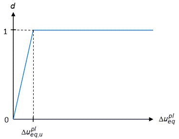
The linear damage-evolution law is defined as:

where  is a material constant representing the relative equivalent plastic
displacement at full degradation
is a material constant representing the relative equivalent plastic
displacement at full degradation  of the material. (See Defining the Ductile-Damage Model.)
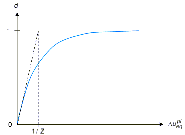
The exponential damage-evolution law is defined as:

where  is a material constant representing the initial slope of this function. (See
Defining the Ductile-Damage Model.)
is a material constant representing the initial slope of this function. (See
Defining the Ductile-Damage Model.)
Setting up a ductile-damage model involves these tasks:
Use native Mechanical APDL small-strain plasticity models in the effective-stress space:
Define the ductile damage-initiation criterion via the damage material data table (TB,CDM,,,,DUCTILE). Enter the damage-initiation threshold vs. stress-triaxiality data points into the table (TBPT):
| Constant | Meaning | Property | Unit | Range |
|---|---|---|---|---|
| X |  | Effective stress triaxiality | --- | --- |
| Y |  | Damage initiation threshold (critical accumulated equivalent plastic strain) | --- |  |
You can define additional dependencies of the damage-initiation threshold on temperature or other field variables (TBTEMP or TBFIELD, respectively).
Damage evolution is either linear or exponential.
Define linear evolution of damage via the damage material data table (TB,CDM,,,,LINDMG) and input the following material constant (TBDATA):
| Constant | Meaning | Property | Unit | Range |
|---|---|---|---|---|
| C1 |  | Relative equivalent plastic displacement at full degradation  | Length | |
Define exponential evolution of damage via the damage material data table (TB,CDM,,,,EXPDMG) and input the following material constant (TBDATA):
| Constant | Meaning | Property | Unit | Range |
|---|---|---|---|---|
| C1 |  | Damage rate coefficient | 1 / Length | |
Define temperature- or field-dependent data for the data tables (TBTEMP or TBFIELD, respectively).
In addition to the crack-band regularization, you can optionally activate viscous regularization for the ductile-damage model to better stabilize the solution.
Define viscous regularization via the damage material table (TB,CDM,,,,VREG) and input the following material constant (TBDATA):
| Constant | Meaning | Property | Unit | Range |
|---|---|---|---|---|
| C1 |  | Characteristic viscous relaxation time | Time | |
If introducing the viscous effect for stabilization only, specify a characteristic viscous-relaxation time that is significantly smaller than the time step of the load step. The smaller time value prevents spurious rate-dependency of the results.
Example 4.51: Defining a Ductile-Damage Model
The following input defines a ductile-damage model combining:
Isotropic linear elasticity
Von Mises plasticity with bilinear isotropic hardening
Stress triaxiality dependent damage initiation threshold
Exponential damage-evolution law
/prep7

! isotropic linear elasticity
TB,ELASTIC,1,,,ISOT
TBDATA,1,70E3 ! Young’s modulus [MPa]
TBDATA,2,0.33 ! Poisson’s ratio [-]

! von Mises plasticity model with bilinear isotropic hardening
TB,PLASTIC,1,,,BISO
TBDATA,1,350  ! initial yield strength [MPa]
TBDATA,2,100  ! plastic tangent modulus [MPa]

! ductile-damage criterion
TB,CDM,1,,,DUCTILE
! stress triaxiality [-], damage initiation threshold [-]
TBPT,DEFI,0.00,1.00
TBPT,DEFI,0.11,0.61
TBPT,DEFI,0.22,0.37
TBPT,DEFI,0.33,0.22
TBPT,DEFI,0.44,0.14
TBPT,DEFI,0.56,0.08
TBPT,DEFI,0.67,0.05
TBPT,DEFI,0.78,0.03
TBPT,DEFI,0.89,0.02
TBPT,DEFI,1.00,0.01

! exponential damage evolution law
TB,CDM,1,,,EXPDMG
TBDATA,1,100 ! initial slope of damage function [1/mm]
Yin, B., Zreid, I., Zhao, D., Ahmed, R., Lin, G., & Kaliske, M. (2022). Thermomechanical fatigue life prediction of metallic materials by a gradient‐enhanced viscoplastic damage approach. International Journal for Numerical Methods in Engineering.. 123(9), 2042-2075.
Yin. B., Zreid, I., Lin, G., Bhashyam, G., & Kaliske, M. (2020). An anisotropic damage formulation for composite materials based on a gradient-enhanced approach: Formulation and implementation at small strain. International Journal of Solids and Structures.
Zreid, I., & Kaliske, M. (2018). A gradient enhanced plasticity-damage microplane model for concrete. Computational Mechanics. 10(1007), 00466-018-1561-1.
Hooputra, H., Gese, H., Dell, H., & Werner, H. (2004). A comprehensive failure model for crashworthiness simulation of aluminium extrusions. International Journal of Crashworthiness. 9(5), 449-464.
Bazant, Z.P., & Oh, B.H. (1983). Crack band theory for fracture of concrete. Materiaux et Constructions. 16(93), 155–177.
[5] Generally,  is identified to be a positive but small value for high-temperature and
fatigue loading.
is identified to be a positive but small value for high-temperature and
fatigue loading.