


The microplane model (TB,MPLANE) is based on research by Bazant and Gambarova [1][2] in which the material behavior is modeled through stress-strain laws on a number of individual planes.
Directional-dependent stiffness degradation is modeled through damage laws on individual potential failure planes, leading to a macroscopic anisotropic damage formulation.
The model is well suited for simulating engineering materials consisting of various aggregate compositions with differing properties (for example, concrete modeling, in which rock and sand are embedded in a weak matrix of cements).
The following microplane material model types are available:
Elastic damage (nonregularized and regularized forms)
Coupled damage-plasticity (regularized form only)
The microplane model cannot be combined with other material models.
The following topics about the microplane model are available:
Also see:
| Material Model Support for Elements |
| Structural Implicit Gradient Regularization in the Coupled-Field Analysis Guide |
Three primary tasks summarize microplane theory:
Apply a kinematic constraint to relate the macroscopic strain tensors to their microplane counterparts (projection).
Define the constitutive laws on the microplane levels, where constitutive equations are applied on each microplane.
Relate the homogenization process on the material point level to derive the overall material response. (Homogenization is based on the principle of energy equivalence.)
The microplane material model formulation is based on the assumption that microscopic free energy Ψmic on the microplane level exists and that the integral of Ψmic over all microplanes is equivalent to a macroscopic free Helmholtz energy Ψmac [3], expressed as:

The factor
 results from
the integration of the sphere of unit radius with respect to the area Ω.
results from
the integration of the sphere of unit radius with respect to the area Ω.
The strains and stresses at microplanes are additively decomposed into volumetric and deviatoric parts, respectively, based on the volumetric-deviatoric (V-D) split.
The strain split is expressed as:

The scalar microplane volumetric strain εv results from:

where V is the second-order volumetric projection tensor and 1 the second-order identity tensor.
The deviatoric microplane strain vector εD is calculated as:

where Π is the fourth-order symmetric identity tensor and the vector n describes the normal on the microsphere (microplane).
The stresses can then be derived by taking the free energy derivative with respect to the strain tensor:

where σv and σ
D are the scalar volumetric
stress and the deviatoric stress tensor on the microsphere, and
 .
.
Assume isotropic elasticity:

and

where Kmic and Gmic are microplane elasticity parameters and can be interpreted as a sort of microplane bulk and shear modulus. They are related to the elastic macroscopic parameters as follows:

|

|
Integration over the surface of the sphere in order to calculate the homogenized quantities is achieved by numerical integration:

where wi is the weight factor.
The following additional topics for microplane modeling are available:
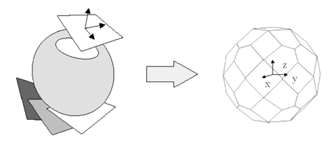
Discretization is the transfer from the microsphere to microplanes which describe the approximate form of the sphere. Forty-two microplanes are used for the numerical integration. Due to the symmetry of the microplanes (where every other plane has the same normal direction), 21 microplanes are considered. [3]
The following figure illustrates the discretization process:
Strain-softening material models often cause mesh sensitivity and numerical instability, a problem mitigated by implicit gradient regularization, a class of nonlocal methods. Implicit gradient regularization enhances a local variable by considering its nonlocal counterpart as an extra degree of freedom governed by a Helmholtz-type equation.
The governing equations are therefore given by the linear momentum-balance equation and a
modified Helmholtz equation describing the nonlocal equivalent strain field  :
:

where  is the Cauchy stress tensor,
  is the body force vector,
  is the divergence,
  is the gradient, and
  is the Laplace operator. The gradient parameter
  controls the range of nonlocal
interaction. The equivalent strain
controls the range of nonlocal
interaction. The equivalent strain  is the local variable to be enhanced, and
  is its nonlocal counterpart.
The homogeneous Neumann boundary condition is used as follows:

where  is the normal to the outer boundary of the nonlocal field. With the
homogeneous Neumann boundary condition, no explicit definition of boundary conditions for the
extra degrees of freedom is required.
is the normal to the outer boundary of the nonlocal field. With the
homogeneous Neumann boundary condition, no explicit definition of boundary conditions for the
extra degrees of freedom is required.
The elastic damage microplane material model is available in nonregularized and regularized forms. The coupled damage-plasticity microplane model is available in a regularized form only.
Identifying the nonlocal interaction-range parameter (related to the length-scale parameter  by the equation
  ) can be somewhat challenging.
One method [8] uses the results comparison of homogeneous
and nonhomogeneous tensile tests of concrete to identify the parameter. The first experiment
consists of a specimen restrained such that the cracking is distributed, while the second
consists of a notched specimen to trigger a localized failure. The damage parameters can be
obtained from homogeneous experiments because, in this case, the damage is uniformly
distributed along the whole specimen and is unaffected by the nonlocal parameter
. In the first step, therefore, the damage parameters are identified from the
stress-strain curve for the homogeneous test. In the second step, the force-displacement curve
for the notched-specimen test identifies the nonlocal parameter , keeping the damage parameters constant.
Other approaches to determine the gradient parameter use the size effects observed in concrete and inverse calibration of
force-deflection curves [9], and calibration based on
fracture-energy test and measurement of crack-surface roughness [10].
The following microplane material model topics are available:
To account for material degradation and damage, the microscopic free-energy function is modified to include a damage parameter, yielding:

The damage parameter dmic is the normalized damage variable
 .
.
The stresses are derived by:

where  and
and  . The stresses derived generally result in unsymmetric material stiffness;
therefore, use the unsymmetric Newton-Raphson solver (NROPT,UNSYM) in such
cases to facilitate convergence.
. The stresses derived generally result in unsymmetric material stiffness;
therefore, use the unsymmetric Newton-Raphson solver (NROPT,UNSYM) in such
cases to facilitate convergence.
The damage status of a material is described by the
equivalent-strain-based damage function  , where ηmic is the equivalent strain, which characterizes the damage evolution law and is defined as:

where I1 is the first invariant of the strain tensor ε, J2 is the second invariant of the deviatoric part of the strain tensor ε, and k0, k1, and k2 are material parameters that characterize the form of damage function. The equivalent strain function implies the Mises-Hencky-Huber criterion for k0 = k1 = 0, and k2 = 1, and the Drucker-Prager-criterion for k0 > 0, k1 = 0, and k2 = 1.
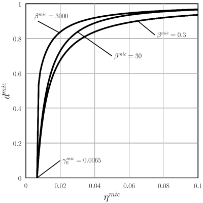
The damage evolution is modeled by the following function:

where α
mic defines the maximal degradation,
βmic determines the rate of damage evolution, and
 is the damage threshold which characterizes the equivalent strain on which the
material damaging starts (damage starting boundary).
is the damage threshold which characterizes the equivalent strain on which the
material damaging starts (damage starting boundary).
 is a history variable representing the largest value of equivalent strain in
the material’s history. The variable is defined differently depending on whether it is
the nonregularized or the regularized version of the elastic damage microplane material model.
Theoretically, the history variable definition is how the two versions differ.
is a history variable representing the largest value of equivalent strain in
the material’s history. The variable is defined differently depending on whether it is
the nonregularized or the regularized version of the elastic damage microplane material model.
Theoretically, the history variable definition is how the two versions differ.
For postprocessing, the maximum damage  is defined as the maximum value of microplane damage values
  . The macroscopic damage is defined by:

and has a range of  .
.
Both nonregularized and regularized versions of the elastic damage microplane material model are available.
The history variable  is calculated as the maximum of the damage threshold and the equivalent strain
  for each microplane:

This figure shows the evolution of the damage variable as a function of equivalent strain  for the implemented exponential damage model:
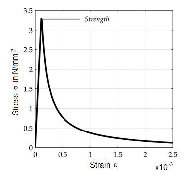
This figure shows the stress-strain behavior for uniaxial tension:
Use the regularized elastic damage microplane model, based on the research by Zreid and Kaliske [6], to overcome the numerical instability and pathological mesh sensitivity to which the nonregularized version of the model is susceptible. The regularized model uses an implicit gradient regularization scheme, defined via a nonlocal field, that adds one extra degree of freedom per node.
The history variable  is calculated as the maximum of the damage threshold and the equivalent strain
  for each microplane:

The modified equivalent strains for each microplane are calculated via implicit gradient regularization.
Implicit Gradient Regularization
The governing equations and boundary condition for the regularized microplane models are included again here for completeness:

where  is the equivalent strain of a given microplane and
  is its nonlocal counterpart. The microplane chosen for
  is the one having the largest equivalent strain
  .
.
The nonlocal counterpart  is obtained as part of solving the system of governing equations shown
above.
is obtained as part of solving the system of governing equations shown
above.
The equivalent strains of each microplane can now be calculated by modifying them with a ratio of local to nonlocal largest equivalent strain:

For more information, see Implicit Gradient Regularization.
The nonregularized elastic damage microplane model requires eight parameters, while the regularized elastic damage microplane model requires nine parameters.
The following elasticity and damage parameters are common to both models and are defined in the same way for both:
| Parameter Type | Parameter | Description | Model | |
|---|---|---|---|---|
| Nonregularized | Regularized | |||
| Elasticity |

| Modulus of elasticity | Y | Y |

| Poisson’s ratio | Y | Y | |
| Damage |

| Damage function material parameters | Y | Y |

| Damage threshold | Y | Y | |

| Maximum damage parameter | Y | Y | |

| Rate of damage evolution | Y | Y | |
| Nonlocal |

| Nonlocal interaction range parameter | N | Y |
Define the elastic parameters and via TB,ELAS or MP.
Define the damage parameters via TB,MPLANE,,,,ORTH.
The following table describes the damage material constants:
| Constant | Meaning |
|---|---|
| C1 |

|
| C2 |

|
| C3 |

|
| C4 |
|
| C5 |
|
| C6 |
|
Considerations for Defining the Nonregularized Model:
Example 4.25: Microplane Material Constant Input
! Define elastic properties of material
tb,elas,1
tbdata,1,60000.0,0.36

! Define microplane model properties
tb,mplane,1,,6,orth
tbdata,1,0,0,1,0.1,0.1,0.1
Considerations for Defining the Regularized Model:
Elements supported: CPT212, CPT213, CPT215, CPT216, and CPT217.
To activate the required extra degree of freedom (GFV1), set KEYOPT(18) = 1. The extra degree of freedom requires no boundary-condition input.
A fine mesh is recommended, particularly at probable damage-prone regions. To observe mesh-independent results, the mesh size may need to be less than half the square root of the nonlocal parameter.
Define the nonlocal parameter via TB,MPLANE,,,,NLOCAL. Following is the material data-table constant:
Constant Meaning C1
Example 4.26: Regularized Elastic Damage Microplane Material Constant Input
/prep7
! Define element
ET,1,215
KEYO,1,18,1  ! Activate extra degree of freedom

! Parameter values
E=18000
nu=.18

k0=0.703125
k1=0.703125
k2=0.2154553289284690
gamma=.0002
alpha=.96
beta=450
c=25

! Define elastic properties of material
mp,ex,1,E
mp,nuxy,1,nu

! Define microplane model properties
tb,mplane,1,,,ORTH
TBDATA,1,k0,k1,k2,gamma,alpha,beta

tb,mplane,1,,,NLOCAL
TBDATA,1,c
Use this model, based on research by Zreid and Kaliske [4][5][6], to overcome the numerical instability and pathological mesh sensitivity to which strain-softening materials such as the microplane model are susceptible.
The model uses an implicit gradient regularization scheme, defined via a nonlocal field, that adds two extra degrees of freedom per node. Microplane plasticity is also introduced, using microplane quantities, through laws resembling classical invariant-based plasticity models, enabling material models with a direct link to the conventional macroscopic plasticity models.
The plasticity in this model is defined via a three-surface microplane Drucker-Prager model, covering a full range of possible stress states and enabling cyclic loading. The damage includes a tension-compression split to account for transition of the stress state during cyclic loading.
To account for coupled damage-plasticity, the microscopic free-energy function is once again modified to include damage; furthermore, the total strain components are additively decomposed into elastic and plastic parts. The resulting stress-strain relation is:

where  is the normalized damage variable
  ,
,  is the volumetric microplane plastic strain, and
  is the deviatoric plastic strain.
The microplane plastic strain rate evolutions are governed by the following flow rules:

|

|
where  is the plastic multiplier, and
  is the given microplane yield function.
The microplane volumetric and deviatoric effective stresses,  and
and  respectively, are defined as:

|

|
The following additional topics about the coupled damage-plasticity microplane model are available:
- 4.10.2.2.1. Smooth Three-Surface Microplane Drucker-Prager Cap Yield Function
- 4.10.2.2.2. Damage Evolution
- 4.10.2.2.3. Implicit Gradient Regularization
- 4.10.2.2.4. Coupled Damage-Plasticity Microplane Model Parameters
- 4.10.2.2.5. Defining the Coupled Damage-Plasticity Microplane Model
- 4.10.2.2.6. Identifying Coupled Damage-Plasticity Microplane Model Parameters
- 4.10.2.2.7. Coupled Damage-Plasticity Microplane Damage Output
A smooth Drucker-Prager yield function with tension and compression caps covers the material response under all possible triaxialities:
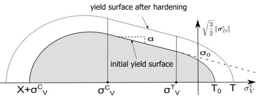
The Drucker-Prager cap model is specific to microplane plasticity, as it uses microplane quantities. It is similar but not identical to the macroscopic Extended Drucker-Prager Cap model. The yield function is expressed as:

where  is the Drucker-Prager yield function with hardening,
  is the compression cap, and
  is the tension cap.
The yield function is evaluated in the undamaged stress space. The product  ensures that the compression cap has the same slope as the function
at the intersection point between
ensures that the compression cap has the same slope as the function
at the intersection point between  and
and  . The same occurs for the tension cap, and so overall the yield surface has
  continuity.
The Drucker-Prager yield function is defined as:

|
where  is the initial yield stress,
  is a friction coefficient, and
  is a hardening function.
The compression cap is defined by:

|

|
where  is the Heaviside step function, and
  is the abscissa of the intersection point between and .
  is the ratio between the major (deviatoric) and minor (volumetric) axes of
the cap. The Heaviside function is used to activate the cap only when the stress state is in
its domain.
is the ratio between the major (deviatoric) and minor (volumetric) axes of
the cap. The Heaviside function is used to activate the cap only when the stress state is in
its domain.
The tension cap is defined by:

|

|
where  is the abscissa of the intersection point between and
  .
.  is the initial intersection of the cap with the volumetric axis, and
 is a hardening parameter controlling the increase of the intersection point
 due to hardening.
The hardening is considered to be linear and is defined by:

|

|
where  is a hardening parameter, and
  is a hardening variable.
The damage evolution behavior is motivated by the material behavior of concrete and similar materials.
To realistically model the damage of concrete subject to cyclic loading, the following considerations are taken into account:
The initiation of damage and its subsequent evolution is different between compression and tension.
Concrete is more brittle in tension, and softening begins to occur almost immediately after the elastic limit.
In compression, some hardening is observed after the elastic limit before softening occurs.
In the transition from tension to compression states, the stiffness lost during tensile cracking is recovered due to crack closure. Upon transition to tension, however, the damage sustained under compression is retained.
This unique behavior is described via a damage split, where the total damage
 is decomposed into compression
  and tension
  parts, as follows:

|

|
where  is the split weight factor,
  represents the principal strain values, and
  indicates the positive principal strain values.
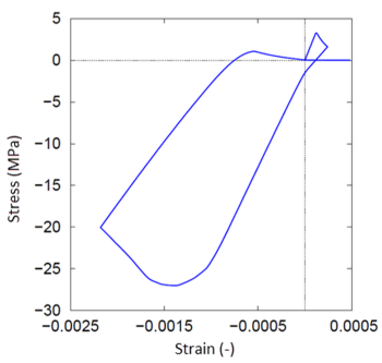
This figure shows the stiffness reduction in unloading and the stiffness recovery in compression:
The damage laws are defined as:

|

|
where  and
and  are material constants.
  and
and  , the variables driving the damage, are calculated from over-nonlocal equivalent strains.
For postprocessing, the homogenized damage  is defined by:

|
Equivalent strain rates  and
and  are functions of the volumetric plastic strain rate, as follows:

|

|
The governing equations and boundary condition are included again here for completeness:
The local variable  and the nonlocal variable
  are both composed of tension and compression parts:

|

|
Each node, therefore, has two extra degrees of freedom.
There are 21 independent values of the equivalent strains  and
and  (one for each microplane). The tension and compression components of the
local variable are evaluated by homogenizing the microplane values, as follows:
(one for each microplane). The tension and compression components of the
local variable are evaluated by homogenizing the microplane values, as follows:

|
The regularization scheme is completed by the over-nonlocal
formulation, where over-nonlocal variables  and
and  are evaluated as a linear combination of local and nonlocal variables, as follows:

|

|
where  is a material parameter which should be > 1 to achieve regularization.
Therefore, the nonlocal variable takes a weight larger than unity and the local variable is
assigned a negative weight (hence the term over-nonlocal). The averaging
ensures a smooth-deformation field, thereby preventing displacement discontinuities which can
lead to an ill-posed boundary-value problem.
is a material parameter which should be > 1 to achieve regularization.
Therefore, the nonlocal variable takes a weight larger than unity and the local variable is
assigned a negative weight (hence the term over-nonlocal). The averaging
ensures a smooth-deformation field, thereby preventing displacement discontinuities which can
lead to an ill-posed boundary-value problem.
The regularized variable is used to calculate the damage driving variables  and
and  , as follows:

|

|
where  and
and  are the tension and compression damage thresholds, respectively.
For more information, see Implicit Gradient Regularization in the Material Reference.
The coupled damage-plasticity microplane model requires 15 parameters:
| Parameter Type | Parameter Subtype | Parameter | Description |
|---|---|---|---|
| Elasticity | -- |

| Modulus of elasticity |
| -- |

| Poisson’s ratio | |
| Plasticity | Drucker-Prager yield function |

| Uniaxial compressive strength |

| Biaxial compressive strength | ||

| Uniaxial tensile strength | ||
| Compression cap |

| Intersection point abscissa between compression cap and Drucker-Prager yield function | |

| Ratio between the major and minor axes of the cap | ||
| Hardening |

| Hardening material constant | |

| Tension cap hardening constant | ||
| Damage | -- |
 , , 
| Tension and compression damage thresholds |
| -- |
 , , 
| Tension and compression damage evolution constants | |
| Nonlocal | -- |

| Nonlocal interaction range parameter |
| -- |

| Over-nonlocal averaging parameter |
The plasticity parameters  ,
,  , and
, and  are used as inputs because they are common material properties (or can be
found experimentally) for materials such as concrete. The initial yield stress
are used as inputs because they are common material properties (or can be
found experimentally) for materials such as concrete. The initial yield stress  and the friction coefficient
  can be calculated by knowing that the biaxial and uniaxial stress states lie
on the linear Drucker-Prager portion of the yield surface as follows:
can be calculated by knowing that the biaxial and uniaxial stress states lie
on the linear Drucker-Prager portion of the yield surface as follows:

|

|
The following empirical relations are used to calculate the tension cap parameters: the
abscissa of the intersection point between the tension cap and the Drucker-Prager yield
function  , and the initial intersection of the cap with the volumetric axis
 :
:

|

|
The coupled damage-plasticity microplane model is used with the following coupled pore-pressure-thermal mechanical solid elements: CPT212, CPT213, CPT215, CPT216, and CPT217.
To activate the required extra degrees of freedom (GFV1, GFV2), set KEYO(18) = 2. The extra degrees of freedom require no boundary condition input.
A fine mesh is recommended, particularly at probable damage-prone regions. To observe
mesh-independent results, the mesh size may need to be less than half the square root of the
nonlocal parameter  .
.
Define the elastic parameters  and
and  via TB,ELAS or MP.
Define the plasticity and damage parameters via TB,MPLANE,,,,DPC. Following are the material data table constants:
| Constant | Meaning | Property | Unit | Range |
|---|---|---|---|---|
| C1 |

| Uniaxial compressive strength | Force/Length2 |

|
| C2 |

| Biaxial compressive strength | Force/Length2 |

|
| C3 |

| Uniaxial tensile strength | Force/Length2 |

|
| C4 |

| Tension cap hardening constant | -- |

|
| C5 |

| Hardening material constant | Force2/Length4 |

|
| C6 |

| Intersection point abscissa between compression cap and Drucker-Prager yield function | Force/Length2 |

|
| C7 |

| Ratio between the major and minor axes of the cap | -- |

|
| C8 |

| Tension damage threshold | -- |

|
| C9 |

| Compression damage threshold | -- |

|
| C10 |

| Tension damage evolution constant | -- |

|
| C11 |

| Compression damage evolution constant | -- |

|
Define the nonlocal parameters via TB,MPLANE,,,,NLOCAL. Following are the material data table constants:
| Constant | Meaning | Property | Unit | Range |
|---|---|---|---|---|
| C1 |

| Nonlocal interaction range parameter | Length2 |

|
| C2 |

| Over-nonlocal averaging parameter | -- |

|
Example 4.27: Coupled Damage-Plasticity Microplane Model Input
/prep7
!Define element
ET,1,215
KEYO,1,18,2  ! Activate extra degrees of freedom

! Parameter values
E = 28000
nu = .2
fuc = 30
fbc = 34.5
fut = 2.9
Rt = 1
D = 4e4
sigVc = -40
R = 2
c = 1500
m = 2.5
gamt0 = 0
gamc0 = 2e-6
betat = .4e4
betac = .25e4

! Define elastic properties of material
MP,EX,1,E
MP,NUXY,1,nu

! Define microplane model properties
TB,MPLA,1,,,DPC
TBDATA,1,fuc,fbc,fut,Rt,D,sigVc
TBDATA,7,R,gamt0,gamc0,betat,betac

TB,MPLA,1,,,NLOCAL
TBDATA,1,c,m
To study a usage example for this material model, see Reinforced Concrete Joint Analysis in the Technology Showcase: Example Problems.
Following are some hints and tips to help you with parameter identification.
Elasticity
 and
and  can be identified from the elastic region of the material stress-strain
curve, or by using empirical formulas available in the literature.
can be identified from the elastic region of the material stress-strain
curve, or by using empirical formulas available in the literature.Plasticity
The strength parameters
 ,
,  , and
, and  are common material properties (or can be found experimentally) for
materials such as concrete. In the absence of complete testing data, empirical relations
[7] can be used if
are common material properties (or can be found experimentally) for
materials such as concrete. In the absence of complete testing data, empirical relations
[7] can be used if  is known:

To identify the compression cap parameters, triaxial experimental data is necessary. The intersection point between the initial compression cap and the hydrostatic axis
 is determined by applying a hydrostatic load until the yielding begins.
 The intersection point between the compression cap and the Drucker-Prager function
 is more challenging to find. It can be approximated as the transition point
from plastic volumetric expansion (occurring on the linear Drucker-Prager function) to
plastic volumetric compaction (occurring on the compression cap). If this data is
unavailable, it can be estimated empirically as:
is more challenging to find. It can be approximated as the transition point
from plastic volumetric expansion (occurring on the linear Drucker-Prager function) to
plastic volumetric compaction (occurring on the compression cap). If this data is
unavailable, it can be estimated empirically as:
The parameter
 (the ratio between the major and minor axes of the cap) can therefore be
calculated as:
(the ratio between the major and minor axes of the cap) can therefore be
calculated as:
Damage and Hardening
To identify the damage and hardening parameters, cyclic tests are necessary. These parameters are related, as their interaction controls the softening and the unloading slope. A uniaxial cyclic compression test identifies the parameters
 ,
,  , and
, and  .
. Similarly, a uniaxial cyclic tension test identifies the parameters
 ,
,  , and
, and  . In the absence of uniaxial cyclic tension tests,
  and
and  can be used as starting values. The tension damage threshold
  is often set to zero, as softening in tension starts almost immediately
after the elastic limit.
is often set to zero, as softening in tension starts almost immediately
after the elastic limit.Nonlocal Parameters
The over-nonlocal averaging parameter
 is a numerical parameter, where
  > 1 regularizes the solution. Typically,
  = 2.5.
Also see Identifying the Nonlocal Interaction-Range Parameter c.
This section applies to both the regularized elastic damage microplane model and the coupled damage-plasticity microplane model.
The Newton-Raphson out-of-balance loads caused by the extra degrees of freedom can be controlled by setting the reference value and tolerance for the gradient field residual (CNVTOL,GFRS).
Example 4.28: Setting the Reference Value and Tolerance for the Gradient Field Residual
CNVTOL,GFRS,1e-7,.001
Automatic time-stepping uses an internal heuristic to adjust the time increment. You can set an additional time-stepping control (CUTCONTROL,MDMG) to limit the maximum allowable microplane homogenized damage increment in a time step.
Bazant, Z. P. & Gambarova, P.G. (1984). Crack shear in concrete: Crack band microplane model. Journal of Structural Engineering. 110, 2015-2036.
Bazant, Z. P. & Oh, B. H. (1985). Microplane model for progressive fracture of concrete and rock. Journal for Engineering Mechanics. 111, 559-582.
Leukart, M. & Ramm, E. (2003). A comparison of damage models formulated on different material scales. Computational Materials Science. 28(3-4), 749-762.
Zreid, I. & Kaliske, M. (2018). A gradient enhanced plasticity-damage microplane model for concrete. Computational Mechanics. 10(1007), s00466-018-1561-1.
Zreid, I. & Kaliske, M. (2016). An implicit gradient formulation for microplane Drucker-Prager plasticity. International Journal of Plasticity. 83, 252-272.
Zreid, I. & Kaliske, M. (2014). Regularization of microplane damage models using an implicit gradient enhancement. International Journal of Solids and Structures. 51(19), 3480-3489.
Jiang, H. & Zhao, J. (2015). Calibration of the continuous surface cap model for concrete. Finite Elements in Analysis and Design. 97, 1-19.
Bažant, Z. P. & Pijaudier-Cabot, G. (1989). Measurement of characteristic length of nonlocal continuum. Journal of Engineering Mechanics. 115(4) 755-767.
Le Bellégo, C., Dubé, J. F., Pijaudier-Cabot, G., & Gérard, B. (2003). Calibration of nonlocal damage model from size effect tests. European Journal of Mechanics-A/Solids. 22(1), 33-46.
Xenos, D., Grégoire, D., Morel, S., & Grassl, P. (2015). Calibration of nonlocal models for tensile fracture in quasi-brittle heterogeneous materials. Journal of the Mechanics and Physics of Solids. 82, 48-60.