


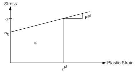
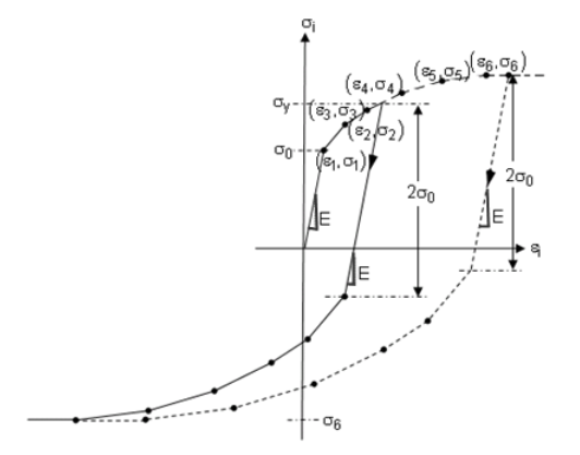
Plasticity is used to model materials subjected to loading beyond their elastic limit. As shown in the following figure, metals and other materials such as soils often have an initial elastic region in which the deformation is proportional to the load, but beyond the elastic limit a nonrecoverable plastic strain develops:
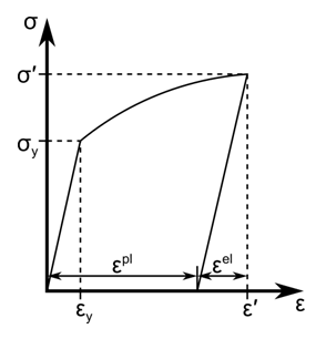
Unloading recovers the elastic portion of the total strain, and if the load is completely removed, a permanent deformation due to the plastic strain remains in the material. Evolution of the plastic strain depends on the load history such as temperature, stress, and strain rate, as well as internal variables such as yield strength, backstress, and damage.
To simulate elastic-plastic material behavior, several constitutive models for plasticity are provided. The models range from simple to complex. The choice of constitutive model generally depends on the experimental data available to fit the material constants.
The following rate-independent plasticity material model topics are available:
The constitutive models for elastic-plastic behavior start with a decomposition of the total strain into elastic and plastic parts and separate constitutive models are used for each. The essential characteristics of the plastic constitutive models are:
The yield criterion that defines the material state at the transition from elastic to elastic-plastic behavior.
The flow rule that determines the increment in plastic strain from the increment in load.
The hardening rule that gives the evolution in the yield criterion during plastic deformation.
The following topics concerning plasticity theory, behavior and model definition are available:
Following are the common symbols used in the rate-independent plasticity theory documentation:
| Symbol | Definition | Symbol | Definition |
|---|---|---|---|
 | Identity tensor |  | Anisotropic directional yield strength |
 | Strain |  | Young's Modulus |
 | Elastic strain |  | Elastoplastic tangent |
 | Plastic strain |  | Elastoplastic tangent in direction i |
 | Plastic strain components |  | Plastic tangent |
 | Effective plastic strain |  | Plastic tangent in direction i |
 | Accumulated equivalent plastic strain |  | Hill yield surface coefficients |
 | Stress |  | Hill yield surface directional yield ratio |
 | Stress components | Reserved | Reserved |
 | Principal stresses | Reserved | Reserved |
 | Stress minus backstress | Reserved | Reserved |
 | Yield stress |  | Plastic work |
 | Anisotropic yield stress in direction i |  | Uniaxial plastic work |
 | Initial yield stress |  | Drucker-Prager yield surface constant |
 | Initial yield stress in direction i |  | Drucker-Prager plastic potential constant |
 | Equivalent plastic stress |  | Mohr-Coulomb cohesion |
 | Von Mises effective stress |  | Mohr-Coulomb internal friction angle |
 | User input strain-stress data point |  | Mohr-Coulomb flow internal friction angle |
 | Magnitude of plastic strain increment |  | Extended Drucker-Prager yield surface pressure sensitivity |
 | Effective stress function |  | Extended Drucker-Prager plastic potential pressure sensitivity |
 | Yield function |  | Extended Drucker-Prager power law yield exponent |
 | Plastic potential |  | Extended Drucker-Prager power law plastic potential exponent |
 | Translation of yield surface (backstress) |  | Extended Drucker-Prager hyperbolic yield constant |
 | Set of material internal variables |  | Extended Drucker-Prager hypobolic plastic potential constant |
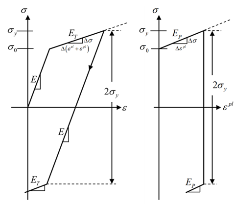
From Figure 4.1: Stress-Strain Curve for an Elastic-Plastic Material , a monotonic loading to  gives a total strain
  . The total strain is additively decomposed into elastic and plastic parts:

The stress is proportional to the elastic strain  :
:

and the evolution of plastic strain  is a result of the plasticity model.
For a general model of plasticity that includes arbitrary load paths, the flow theory of plasticity decomposes the incremental strain tensor into elastic and plastic strain increments:

The increment in stress is then proportional to the increment in elastic strain, and the plastic constitutive model gives the incremental plastic strain as a function of the material state and load increment.
The yield criterion is a scalar function of the stress and internal variables and is given by the general function:
 | (4–4) |
where  represents a set of history dependent scalar and tensor internal variables.
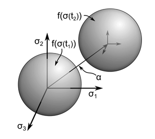
Equation 4–4 is a general function representing the specific form of the yield criterion for each of the plasticity models. The function is a surface in stress space and an example, plotted in principal stress space, as shown in this figure:
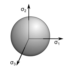
Stress states inside the yield surface are given by  and result in elastic deformation. The material yields when the stress state reaches the yield surface and further
loading causes plastic deformation. Stresses outside the yield surface do not exist and the plastic strain and shape of the yield
surface evolve to maintain stresses either inside or on the yield surface.
and result in elastic deformation. The material yields when the stress state reaches the yield surface and further
loading causes plastic deformation. Stresses outside the yield surface do not exist and the plastic strain and shape of the yield
surface evolve to maintain stresses either inside or on the yield surface.
The evolution of plastic strain is determined by the flow rule:

where  is the magnitude of the plastic strain increment and
  is the plastic potential.
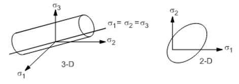
When the plastic potential is the yield surface from Equation 4–4 , the plastic strain increment is normal to the yield surface and the model has an associated flow rule, as shown in this figure:
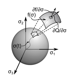
These flow rules are typically used to model metals and give a plastic strain increment that is proportional to the stress increment. If the plastic potential is not proportional to the yield surface, the model has a non-associated flow rule, typically used to model soils and granular materials that plastically deform due to internal frictional sliding. For non-associated flow rules, the plastic strain increment is not in the same direction as the stress increment.
Non-associated flow rules result in an unsymmetric material stiffness tensor. Unsymmetric analysis can be set via the NROPT command. For a plastic potential that is similar to the yield surface, the plastic strain direction is not significantly different from the yield surface normal, and the degree of asymmetry in the material stiffness is small. In this case, a symmetric analysis can be used, and a symmetric material stiffness tensor will be formed without significantly affecting the convergence of the solution.
The yield criterion for many materials depends on the history of loading and evolution of plastic strain. The change in the yield criterion due to loading is called hardening and is defined by the hardening rule. Hardening behavior results in an increase in yield stress upon further loading from a state on the yield surface so that for a plastically deforming material, an increase in stress is accompanied by an increase in plastic strain.
Two common types of hardening rules are isotropic and kinematic hardening. For isotropic hardening, the yield surface given by Equation 4–4 has the form:

where  is a scalar function of stress and
  is the yield stress.
Plastic loading from  to
to  increases the yield stress and results in uniform increase in the size of the yield surface, as shown in this
figure:
increases the yield stress and results in uniform increase in the size of the yield surface, as shown in this
figure:
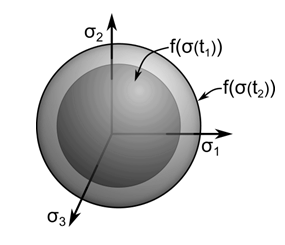
This type of hardening can model the behavior of materials under monotonic loading and elastic unloading, but often does not give good results for structures that experience plastic deformation after a load reversal from a plastic state.
For kinematic hardening, the yield surface has the form:

where  is the backstress tensor.
As shown in the following figure, the backstress tensor is the center (or origin) of the yield surface, and plastic loading from
 to
to  results in a change in the backstress and therefore a shift in the yield surface:
Kinematic hardening is observed in cyclic loading of metals. It can be used to model behavior such as the Bauschinger effect, where the compressive yield strength reduces in response to tensile yielding. It can also be used to model plastic ratcheting, which is the buildup of plastic strain during cyclic loading.
Many materials exhibit both isotropic and kinematic hardening behavior, and these hardening rules can be used together to give the combined hardening model. Other hardening behaviors include changes in the shape of the yield surface in which the hardening rule affects only a local region of the yield surface, and softening behavior in which the yield stress decreases with plastic loading.
The plasticity constitutive models are applicable in both small-deformation and large-deformation analyses. For small deformation, the formulation uses engineering stress and strain. For large deformation (NLGEOM ,ON), the constitutive models are formulated with the Cauchy stress and logarithmic strain.
Input quantities (such as the stress versus strain points for the multilinear isotropic hardening model) and output quantities (such as stress and elastic strain) use the stress and strain measures that correspond to the nonlinear geometry setting (NLGEOM).
Output quantities specific to the plastic constitutive models are available for use in the POST1 database postprocessor (/POST1) and in the POST26 time-history results postprocessor (/POST26).
The equivalent stress (label SEPL) is the current value of the yield stress evaluated from the hardening model.
The accumulated plastic strain (label EPEQ) is a path-dependent summation of the plastic strain rate over the history of the deformation:


where  is the magnitude of the plastic strain increment.
The stress ratio (label SRAT) is the ratio of the elastic trial stress to the current yield stress and is an indicator of plastic deformation during an increment. If the stress ratio is:
- > 1
A plastic deformation occurred during the increment.
- < 1
An elastic deformation occurred during the increment.
- 1
The stress state is on the yield surface.
Hill, R. (1983). The Mathematical Theory of Plasticity . New York: Oxford University Press.
Prager, W. (1955). The theory of plasticity: A Survey of recent achievements. Proceedings of the Institution of Mechanical Engineers. 169(1), 41-57.
Besseling, J. F. (1958). A theory of elastic, plastic, and creep deformations of an initially isotropic material showing anisotropic strain-hardening, creep recovery, and secondary creep. ASME Journal of Applied Mechanics. 25, 529-536.
Owen, D. R. J., Prakash, A., & Zienkiewicz, O. C. (1974) Finite element analysis of nonlinear composite materials by use of overlay systems. Computers and Structures. 4(6), 1251-1267.
Rice, J. R. (1975). Continuum mechanics and thermodynamics of plasticity in relation to microscale deformation mechanisms. Argon, A. (Ed.). Constitutive Equations in Plasticity . 23-79.
Chaboche, J. L. (1989) Constitutive equations for cyclic plasticity and cyclic viscoplasticity. International Journal of Plasticity. 5(3), 247-302.
Chaboche, J. L. (1991). On some modifications of kinematic hardening to improve the description of ratchetting effects. International Journal of Plasticity. 7(7), 661-678.
Chaboche, J. L. (2008). A review of some plasticity and viscoplasticity constitutive theories. International Journal of Plasticity. 24(10), 1642-1693.
Shih, C. F. & Lee, D. (1978). Further developments in anisotropic plasticity. Journal of Engineering Materials and Technology. 100(3), 294-302.
Valliappan, S., Boonlaulohr, P., & Lee, I. K. (1976). Nonlinear analysis for anisotropic materials. International Journal for Numerical Methods in Engineering. 10(3), 597-606.
Sandler, I. S., DiMaggio, F. L., & Baladi, G. Y. (1976). A generalized cap model for geological materials. Journal of the Geotechnical Engineering Division. 102(7), 683-699.
Schwer, L. E. & Murray, Y. D. (1994). A three-invariant smooth cap model with mixed hardening. International Journal for Numerical and Analytical Methods in Geomechanics. 18(10), 657-688.
Foster, C., Regueiro, R., Fossum, A., & Borja, R. (2005). Implicit numerical integration of a three-invariant, isotropic/kinematic hardening cap plasticity model for geomaterials. Computer Methods in Applied Mechanics and Engineering. 194(50-52), 5109-5138.
Pelessone, D. (1989). A modified formulation of the cap model. Technical Report GA-C19579. San Diego: Gulf Atomics.
Fossum, A.F. & Fredrich, J. T. (2000). Cap plasticity models and compactive and dilatant pre-failure deformation. Girard, J., Liebman, M., Breeds, C., Doe, T., & Balkema, A. A. (Eds.). (pp. 1169-1176). Proceedings of the Fourth North American Rock Mechanics Symposium. Pacific Rocks 2000: Rock Around the Rim. Rotterdam.
Gurson, A. L. (1977). Continuum theory of ductile rupture by void nucleation and growth: Part I--yield criteria and flow rules for porous ductile media. Journal of Engineering Materials and Technology. 99(1), 2-15.
Needleman, A. & Tvergaard, V. (1984). An analysis of ductile rupture in notched bars. Journal of the Mechanics and Physics of Solids. 32(6), 461-490.
Arndt, S., Svendsen, B., & Klingbeil, D. (1997). Modellierung der Eigenspannungen an der Riβspitze mit einem Schädigungsmodell. Technische Mechanik. 4(17), 323-332.
Besson, J. & Guillemer-Neel, C. (2003). An extension of the green and gurson models to kinematic hardening. Mechanics of Materials. 35(1-2), 1-18.
Hjelm, H. E. (1994). Yield surface for grey cast iron under biaxial stress. Journal of Engineering Materials and Technology. 116(2), 148-154.
Chen, W. F. & Han, D. J. (1998). Plasticity for Structural Engineers. New York: Springer-Verlag.
Mϋhlich, U. and Brocks, W. (2003). On the numerical integration of a class of pressure-dependent plasticity models including kinematic hardening. Computational Mechanics. 31(6), 479-488.
Mechanical APDL offers two anisotropic material model options:
Hill potential theory (TB ,HILL)
Generalized Hill potential theory (TB ,ANISO)
Anisotropic Hill potential theory (TB ,HILL) uses Hill's [ 1 ] criterion (an extension to the von Mises yield criterion) to account for the anisotropic yield of the material. When this criterion is used with the isotropic hardening option, the yield function is given by:
 | (4–5) |
where:
 = reference yield stress = reference yield stress |
 = equivalent plastic strain = equivalent plastic strain |
and when used with the kinematic hardening option, the yield function takes the form:
 | (4–6) |
The material is assumed to have three orthogonal planes of symmetry. Assuming the material coordinate system is perpendicular to
these planes of symmetry, the plastic compliance matrix  can be written as:
 | (4–7) |
 ,
,  ,
,  ,
,  ,
,  , and
, and  are material constants that can be determined experimentally. They are defined as:
 | (4–8) |
 | (4–9) |
 | (4–10) |
 | (4–11) |
 | (4–12) |
 | (4–13) |
The yield stress ratios  ,
,  ,
,  ,
,  ,
,  and
and  are user-specified and are calculated as:
 | (4–14) |
 | (4–15) |
 | (4–16) |
 | (4–17) |
 | (4–18) |
 | (4–19) |
where:
 = yield stress values = yield stress values |
Two notes:
The inelastic compliance matrix should be positive definite in order for the yield function to exist.
The plastic slope (see also Equation 4–42) is calculated as:
 | (4–20) |
where:
 = elastic modulus in the x direction = elastic modulus in the x direction |
 = tangent modulus defined by the hardening input = tangent modulus defined by the hardening input |
After defining the material data table (TB ,HILL), input the required constants (TBDATA):
| Constant | Meaning | Property |
|---|---|---|
| C1 | R 11 | Yield stress ratio in X direction |
| C2 | R 22 | Yield stress ratio in Y direction |
| C3 | R 33 | Yield stress ratio in Z direction |
| C4 | R 12 | Yield stress ratio in XY direction |
| C5 | R 23 | Yield stress ratio in YZ direction |
| C6 | R 13 | Yield stress ratio in XZ direction |
The constants can be defined as a function of temperature
(NTEMP on TB), with temperatures
specified for the table entries (TBTEMP).
Example 4.2: Defining the Data Table for the Hill Model
/prep7
MP,EX,1,20.0E5                   ! ELASTIC CONSTANTS
MP,NUXY,1,0.3
TB,HILL,1                        ! HILL TABLE
TBDATA,1,1.0,1.1,0.9,0.85,0.9,0.80
Generalized Hill potential theory (TB ,ANISO), an extension of Hill's formulation,[ 1 ] allows for differing stress-strain behavior in the material x, y, and z directions, and differing tension and compression behavior. A Hill yield criterion is used to determine yielding.
This option is not recommended for cyclic or highly nonproportional load histories, as work hardening is assumed. The principal axes of anisotropy coincide with the material (or element) coordinate system and are assumed not to change over the load history.
The material behavior is described by the uniaxial tensile and compressive stress-strain curves in three orthogonal directions, and the shear stress-engineering shear strain curves in the corresponding directions. A bilinear response in each direction is assumed. The initial slope of the curve is taken as the elastic moduli of the material. At the specified yield stress, the curve continues along the second slope defined by the tangent modulus (having the same units as the elastic modulus). The tangent modulus cannot be less than zero or greater than the elastic modulus.
All values must be specified, as no defaults are defined. Input the magnitude of the yield stresses (without signs). No yield stress can have a zero value. The tensile x direction serves the reference curve for output quantities SEPL and EPEQ.
Temperature-dependent curves cannot be specified.
The generalized Hill model supports current-technology elements only.
The following topics are available:
After initializing the stress-strain table (TB ,ANISO), define up to 18 constants (TBDATA):
| Constant | Meaning | Property |
|---|---|---|
| C1-C3 |  | Tensile yield stresses in the material x, y, and z directions. |
| C4-C6 |  | Corresponding tangent moduli. |
| C7-C9 |  | Compressive yield stresses in the material x, y, and z directions. |
| C10-C12 |  | Corresponding tangent moduli. |
| C13-C15 |  | Shear yield stresses in the material xy, yz, and xz directions. |
| C16-C18 |  | Corresponding tangent moduli. |
Example 4.3: Defining the Data Table for the Generalized Hill Model
! Define elasticity data table
TB,ELASTIC,1,,9,OELN
TBDATA,1,EX,EY,EZ
TBDATA,4,GXY,GYZ,GXZ
TBDATA,7,NUYX,NUZY,NUZX
! Define Generalized Hill data table
TB,ANISO,1
TBDATA,1,10000,12000,9000,2e6,1e6,2e6
TBDATA,7,12000,14000,7159.1,1e6,2e6,4e6
TBDATA,13,5000,7000,8000,1e6,2e6,1e6
Generalized anisotropic Hill potential theory uses Hill's [ 1 ] yield criterion to account for differences in yield strengths in orthogonal directions, but is modified (Shih and Lee [ 9 ]) to also account for differences in yield strength in tension and compression. An associated flow rule is assumed. Work hardening (as presented by Valliappan et al. [ 10 ]) is used to update the yield criterion. The yield surface is therefore a distorted circular cylinder that is initially shifted in stress space which expands in size with plastic straining.
The equivalent stress for the generalized Hill option is redefined as:

where  is a matrix describing the variation of the yield stress with orientation, and
  accounts for the difference between tension and compression yield strengths.
 can be related to the yield surface translation for kinematic hardening.[ 9 ] The
equivalent stress function can therefore be interpreted as having an initial translation or shift. When
can be related to the yield surface translation for kinematic hardening.[ 9 ] The
equivalent stress function can therefore be interpreted as having an initial translation or shift. When  equals a material parameter
  , the material is assumed to yield.
The yield criterion is then:
 | (4–21) |
The material is assumed to have three orthogonal planes of symmetry. The plastic behavior can then be characterized by the
stress-strain behavior in the three element coordinate directions and the corresponding shear stress-shear strain behavior.
Therefore, has the form:

By evaluating the yield criterion Equation 4–21 for all possible uniaxial stress conditions, the individual terms of [M] can be identified:
 | (4–22) |
where  and
and  = tensile and compressive yield strengths in direction
 (
( = 1 to 6).
Compressive yield stress is handled as a positive number here. For the shear yields,  =
=  . Letting
  = 1 defines
  to be:

The strength differential vector  has the form:

and from the uniaxial conditions,  is defined as:
 | (4–23) |
Assuming plastic incompressibility (no increase in material volume due to plastic straining) yields the following relationships:

and
 | (4–24) |
The off-diagonals are therefore:

Note that Equation 4–24 (via Equation 4–22 and Equation 4–23) yields the consistency equation:

that must be satisfied due to the requirement of plastic incompressibility. The uniaxial yield strengths are therefore not completely independent.
The yield strengths must also define a closed yield surface (that is, elliptical in cross-section). An elliptical yield surface is defined if the following criterion is met:

The criterion further restricts the independence of the uniaxial yield strengths. Because the yield strengths change with plastic straining (a consequence of work hardening), this condition must be satisfied throughout the loading history. The program checks the condition using an equivalent plastic strain level of 20 percent (.20).
For an isotropic material,

and

and the yield criterion (Equation 4–21) reduces to the von
Mises yield criterion  .
.
Work hardening is used for the hardening rule so that the subsequent yield strengths increase with increasing total plastic work done on the material. The increment in plastic work is:

where  = the average stress over the increment.
For the uniaxial case, the total plastic work is simply:
 | (4–25) |
where the terms are defined as shown in Figure 4.6: Yield Surface for Hill Yield Criterion .
The bilinear stress-strain behavior is:
 | (4–26) |
where:
 = plastic slope = plastic slope |
 = elastic modulus = elastic modulus |
 = tangent modulus = tangent modulus |
Combining Equation 4–26 with Equation 4–25 and solving for the updated yield stress  :
:

Extending this result to the anisotropic case gives:
 | (4–27) |
where  refers to each of the input stress-strain curves.
Equation 4–27 determines the updated yield stresses by equating the amount of plastic work done on the material to an equivalent amount of plastic work in each of the directions.
The parameters  and
and  can then be updated from their definitions (Equation 4–22 and Equation 4–23) and the new values of the
yield stresses. For isotropic materials, this hardening rule reduces to the case
of isotropic hardening.
can then be updated from their definitions (Equation 4–22 and Equation 4–23) and the new values of the
yield stresses. For isotropic materials, this hardening rule reduces to the case
of isotropic hardening.
The equivalent plastic strain  (output as EPEQ) is determined using the tensile x direction as the reference axis by substituting Equation 4–26 into Equation 4–25 :

where the yield stress in the tensile x direction  refers to the initial (not updated) yield stress.
The equivalent stress parameter (output as SEPL) is defined as:

where again  is the initial yield stress.
During plastic deformation, isotropic hardening causes a uniform increase in the size of the yield surface and results in an increase in the yield stress. The yield criterion has the form:

where  is a scalar function of stress and
  is the yield stress that evolves as a function of the set of material internal variables
  . This type of hardening can model the behavior of materials under monotonic loading and elastic unloading, but often
does not give good results for structures that experience additional plastic deformation after a load reversal from a plastic state.
. This type of hardening can model the behavior of materials under monotonic loading and elastic unloading, but often
does not give good results for structures that experience additional plastic deformation after a load reversal from a plastic state.
Three general classes of isotropic hardening models are available: bilinear, multilinear, and nonlinear. Each of the hardening models assumes a von Mises yield criterion , unless an anisotropic Hill yield criterion is defined, and includes an associated flow rule.
Isotropic hardening can also be combined with kinematic hardening and the Extended Drucker-Prager and Gurson models to provide an evolution of the yield stress. For more information, see Combining Material Models .
The following topics concerning the isotropic hardening material model are available:
Hardening models assume a von Mises yield criterion, unless an anisotropic Hill yield criterion is defined.
The von Mises yield criterion is commonly used in plasticity models for a wide range of materials. It is a good first approximation for metals, polymers, and saturated geological materials. The criterion is isotropic and independent of hydrostatic pressure, which can limit its applicability to microstructured materials and materials that exhibit plastic dilatation.
The von Mises yield criterion is:
 | (4–28) |
where  is the von Mises effective stress, also known as the von Mises equivalent stress,

and  is the yield strength and corresponds to the yield in uniaxial stress loading.
In principal stress space, the yield surface is a cylinder with the axis along the hydrostatic line  and gives a yield criterion that is independent of the hydrostatic stress, as shown in the following figure:
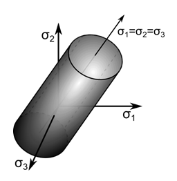
For an associated flow rule, the plastic potential is the yield criterion in Equation 4–28 and the plastic strain increment is proportional to the deviatoric stress

The anisotropic Hill yield criterion [ 1 ] depends on the orientation of the stress relative to the axis of anisotropy. It can be used to model materials in which the microstructure influences the macroscopic behavior of the material such as forged metals and composites.
In a coordinate system that is aligned with the anisotropy coordinate system, the Hill yield criterion given in stress components is:
 | (4–29) |
The coefficients in this yield criterion are functions of the ratio of the scalar yield stress parameter and the yield stress in each of the six stress components:

where the directional yield stress ratios are the user-input parameters and are related to the isotropic yield stress parameter by:

where  is the yield stress in the direction indicated by the value of
subscript i. The stress directions are in the anisotropy coordinate system which
is aligned with the element coordinate system (ESYS). The
isotropic yield stress
is the yield stress in the direction indicated by the value of
subscript i. The stress directions are in the anisotropy coordinate system which
is aligned with the element coordinate system (ESYS). The
isotropic yield stress  is entered in the constants for the hardening model.
The Hill yield criterion defines a surface in six-dimensional stress space and the flow direction is normal to the surface. The plastic strain increments in the anisotropy coordinate system are:

The Hill surface, used with a hardening model, replaces the default von Mises yield surface.
For information about defining the Hill model, see Hill Anisotropy .
This capability is reserved for use with the material combination of Chaboche nonlinear kinematic hardening with implicit creep.
To define separated Hill potentials for the plastic yielding and the creep flow (TB ,HILL,,,,PC), issue two TBDATA commands, one to set constants C1-C6 defining the Hill yield surface for plasticity, the other to set constants C7-C12 defining the Hill potential for the creep direction.
Example 4.4: Defining Hill Surfaces for Plasticity and Creep
/prep7
MP,EX,1,20.0E5                     ! ELASTIC CONSTANTS
MP,NUXY,1,0.3
TB,HILL,1,1,,PC                    ! HILL data table for plasticity and creep
TBDATA,1,1.0,1.1,0.9,0.85,0.9,0.80 ! Plasticity Hill parameters
TBDATA,7,1.0,1.0,1.0,1.0 ,1.0,1.0  ! Creep Hill parameters
Support is available for these general classes of isotropic hardening:
Bilinear isotropic hardening is described by a bilinear effective-stress versus effective-strain curve. The initial slope of
the curve is the elastic modulus of the material. Beyond the user-specified initial yield stress  , plastic strain develops and stress-vs.-total-strain continues along a line with slope equal to the tangent
modulus
, plastic strain develops and stress-vs.-total-strain continues along a line with slope equal to the tangent
modulus  .
.
In effective-stress vs. effective-plastic-strain space, bilinear isotropic hardening is described by a line initially
intersecting the stress axis at  and continuing with the slope of the user-defined plastic tangent modulus
  . The plastic tangent modulus cannot be less than zero.
The tangent modulus  and the plastic tangent modulus
  are related by:

where  is the elastic modulus.
Figure 4.9: Stress vs. Total Strain (a), and Stress vs. Plastic Strain (b) for Bilinear Isotropic Hardening
Define the isotropic or anisotropic elastic behavior via MP or TB .
Define bilinear isotropic hardening by providing the plastic tangent
modulus  (TB ,PLAS,,,,BISO).
The constants can be defined as a function of temperature with temperatures specified for the table entries (TBTEMP or TBFIELD ,TEMP).
Defining the Bilinear Isotropic Hardening Model
After defining the material data table (TB ,PLAS,,,,BISO), input the following constants (TBDATA):
| Constant | Meaning | Property |
|---|---|---|
| C1 |  | Yield stress |
| C2 | | Plastic tangent modulus |
Example 4.5: Bilinear Isotropic Hardening
/prep7
MPTEMP,1,0,500            ! Define temperatures for Young's modulus
MPDATA,EX,1,,14E6,12e6
MPDATA,PRXY,1,,0.3,0.3
TB,PLAS,1,2,,BISO         ! Activate a data table
TBTEMP,0.0                ! Temperature = 0.0
TBDATA,1,44E3,1.2E6       ! Yield = 44,000; Plastic Tangent modulus = 1.2E6
TBTEMP,500                ! Temperature = 500
TBDATA,1,29.33E3,0.8E6    ! Yield = 29,330; Plastic Tangent modulus = 0.8E6
The behavior of multilinear isotropic hardening is similar to bilinear isotropic hardening except that a multilinear stress versus total or plastic strain curve is used instead of a bilinear curve.
The multilinear hardening behavior is described by a piece-wise linear stress-total strain curve, starting at the origin and defined by sets of positive stress and strain values, as shown in this figure:
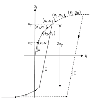
The first stress-strain point corresponds to the yield stress. Subsequent points define the elastic plastic response of the material.
Define the isotropic or anisotropic elastic behavior via MP commands. After defining the material data table (TB ,PLASTIC,,,,MISO), input the following constants (TBDATA):
| Constant | Meaning | Property |
|---|---|---|
| X |  | Plastic strain value |
| Y |  | Stress value |
The stress-plastic strain data points are entered into the table via the TBPT command.
By default, the program error traps for negative tangent slopes of the stress-strain curve. To allow negative tangent slopes, issue TBEO ,NEGSLOPE,1.
Define a sufficient number of table points to cover the range of multilinear hardening behavior. If the accumulated equivalent plastic-strain value exceeds the bounds of the defined table, Mechanical APDL uses the nearest table point. This behavior results in the hardening curve being perfectly plastic beyond the last-defined data point.
Temperature-dependent data can be defined
(NTEMP on the TB command),
with temperatures specified for the table entries
(TBTEMP). Interpolation between temperatures occurs via
stress-vs.-plastic-strain.
Example 4.6: Multilinear Hardening with Plastic Strain
/prep7
MPTEMP,1,0,500            ! Define temperature-dependent EX,
MPDATA,EX,1,,14.665E6,12.423e6
MPDATA,PRXY,1,,0.3
TB,PLASTIC,1,2,5,MISO     ! Activate TB,PLASTIC data table
TBTEMP,0.0                ! Temperature = 0.0
TBPT,DEFI,0,29.33E3       ! Plastic strain, stress at temperature = 0
TBPT,DEFI,1.59E-3,50E3
TBPT,DEFI,3.25E-3,55E3
TBPT,DEFI,5.91E-3,60E3
TBPT,DEFI,1.06E-2,65E3
TBTEMP,500                ! Temperature = 500
TBPT,DEFI,0,27.33E3       ! Plastic strain, stress at temperature = 500
TBPT,DEFI,2.02E-3,37E3
TBPT,DEFI,3.76E-3,40.3E3
TBPT,DEFI,6.48E-3,43.7E3
TBPT,DEFI,1.12E-2,47E3
The power law equation has a user-defined initial yield stress  and exponent N. The current yield stress
  is given by solving the following equation:

where G is the shear modulus determined from the user-defined elastic constants and  is the accumulated equivalent plastic strain.
Defining the Power Law Nonlinear Isotropic Hardening Model
For the power law hardening model, define the isotropic or anisotropic elastic behavior via MP commands. After defining the material data table (TB ,NLISO,,,,POWER), input the following constants (TBDATA):
| Constant | Meaning | Property |
|---|---|---|
| C1 |  | Initial yield stress |
| C2 | N | Exponent |
The exponent N must be positive and less than 1.
Temperature-dependent data can be defined
(NTEMP on the TB command),
with temperatures specified for the subsequent set of constants
(TBTEMP).
Example 4.7: Power Law Nonlinear Isotropic Hardening
/prep7
TB,NLISO,1,2,,POWER
TBTEMP,100               ! Define first temperature
TBDATA,1,275,0.1
TBTEMP,200               ! Define second temperature
TBDATA,1,275,0.1
The Voce hardening model is similar to bilinear isotropic hardening, with an exponential saturation hardening term added to the linear term, as shown in this figure:
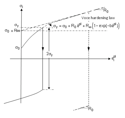
The evolution of the yield stress for this model is specified by the following equation:

where the user-defined parameters include  , the difference between the saturation stress and the initial yield stress,
  , the slope of the saturation stress and,
  , the hardening parameter that governs the rate of saturation of the exponential term.
Defining the Voce Law Nonlinear Isotropic Hardening Model
Define the isotropic or anisotropic elastic behavior via MP commands. After defining the material data table (TB ,NLISO,,,,VOCE), input the following constants (TBDATA):
| Constant | Meaning | Property |
|---|---|---|
| C1 |  | Initial yield stress |
| C2 |  | Linear coefficient |
| C3 |  | Exponential coefficient |
| C4 |  | Exponential saturation parameter |
The constants can be defined as a function of temperature
(NTEMP on the TB command),
with temperatures specified for the subsequent set of constants
(TBTEMP).
Example 4.8: Voce Nonlinear Isotropic Hardening
/PREP7
TB,NLISO,1,2,,VOCE         ! Activate NLISO data table
TBTEMP,40                  ! Define first temperature
TBDATA,1,280,7e3,155,7e2   ! Constants at first temperature
TBTEMP,60                  ! Define second temperature
TBDATA,1,250,5e3,120,3e2   ! Constants at second temperature
Static recovery, also known as thermal recovery, of the isotropic yield stress is dependent on time, temperature and the current yield stress. The rate of isotropic hardening can be separated into work hardening and static recovery, as follows:

where the first term on the right side of the equation represents the rate of work hardening, and the second defines the rate
of static recovery where  ,
,  and
and  are material parameters,
  is the temperature, and
  is the current yield stress. A lower limit yield stress can be defined for static recovery such that:

where  is the user-defined static recovery threshold.
An approximate solution for the static recovery of the yield stress over a time step is to integrate the static recovery rate and incorporate the work hardening rate into the initial condition. The yield stress is then given by the solution to:

with the initial condition:

where  is the yield stress at the end of the previous increment and
  is the increment in yield stress due to work hardening over the current time step.
Static recovery of the isotropic yield stress can be used with the combined creep and Chaboche nonlinear hardening
material. The material parameters are defined via a TB material table with Lab =
PLASTIC and TBOPT = ISR.
| Constant | Meaning | Property |
|---|---|---|
| C1 |  | Coefficient |
| C2 |  | Temperature Coefficient |
| C3 |  | Exponential |
| C4 |  | Recovery threshold |
The constants can be defined as a function of temperature
(NTEMP on the TB command),
with temperatures specified for the table entries
(TBTEMP).
Example 4.9: Isotropic Hardening Static Recovery
/prep7
YOUNGS = 30e3   ! Young’s Modulus
NU     = 0.3    ! Poisson’s ratio
SIGMA0 = 18.0E0 ! Initial yield stress

mp,ex,1,YOUNGS
mp,prxy,1,NU
TB,CHAB,1,1,1    ! Chaboche kinematic hardening
TBDATA,1,sigma0,
TBDATA,2,1e+3,0
TB,CREEP,1,1, ,1,1   ! creep model
tbdata,1,            ! No creep strain
TB,PLASTIC,1,,,MISO  ! Multilinear isotropic hardening
TBPT,DEFI,0.0,SIGMA0
TBPT,DEFI,0.001,35.0
TBPT,DEFI,0.002,40.0
TBPT,DEFI,0.010,60.0
TB,PLASTIC,1,,4,ISR  ! Isotropic hardening static recovery
TBDATA,1,1D-5,1,2,SIGMA0
During plastic deformation, kinematic hardening causes a shift in the yield surface in stress space. In uniaxial tension, plastic deformation causes the tensile yield stress to increase and the magnitude of the compressive yield stress to decrease. This type of hardening can model the behavior of materials under either monotonic or cyclic loading and can be used to model phenomena such as the Bauschinger effect and plastic ratcheting.
The yield criterion has the form:

where  is a scalar function of the relative stress
  and
and  is the yield stress. The relative stress is:
 | (4–30) |
where the backstress  is the shift in the position of the yield surface in stress space and evolves during plastic deformation.
The general classes of kinematic hardening models are bilinear, multilinear, and nonlinear. The hardening models assume a von Mises yield criterion , unless an anisotropic Hill yield criterion is defined, and includes an associated flow rule.
Kinematic hardening can also be combined with isotropic hardening and the Gurson model to provide an evolution of the yield stress. For more information, see Combining Material Models.
The following topics concerning the kinematic hardening material model are available:
Kinematic hardening uses the von Mises yield criterion with an associated flow rule unless a Hill yield surface is defined. If a Hill yield surface is defined, the kinematic hardening model uses it for both the yield criterion and as the plastic potential to give an associated flow rule.
For more information about von Mises and Hill yield surfaces, see Yield Criteria and Plastic Potentials .
Support is available for these general classes of kinematic hardening:
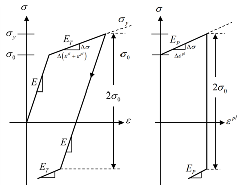
The backstress tensor for bilinear kinematic hardening evolves so that the effective stress versus effective strain curve is
bilinear. The initial slope of the curve is the elastic modulus of the material and beyond the user-specified initial yield stress
 , plastic strain develops and the backstress evolves so that stress versus total strain continues along a line
with slope equal to the tangent modulus
, plastic strain develops and the backstress evolves so that stress versus total strain continues along a line
with slope equal to the tangent modulus  .
.
In effective-stress vs. effective-plastic-strain space, bilinear kinematic hardening is described by a line initially
intersecting the stress axis at and continuing with the slope of the user-defined plastic tangent modulus . The plastic tangent modulus cannot be less than zero.
The tangent modulus and the plastic tangent modulus are related by:
where is the elastic modulus.
For uniaxial tension followed by uniaxial compression, the magnitude of the compressive yield stress decreases as the tensile
yield stress increases so that the magnitude of the elastic range is always  , as shown in this figure:
Figure 4.12: Stress vs. Total Strain (a), and Stress vs. Plastic Strain (b) for Bilinear Kinematic Hardening
For non-isothermal loading, Rice's hardening rule is applied, which accounts for stress relaxation with temperature increase.
The backstress is proportional to the shift strain  :
:

where G is the elastic shear modulus and the shift strain is numerically integrated from the incremental shift strain which is proportional to the incremental plastic strain:

where

and  is Young's Modulus,
  is the user-defined tangent modulus [ 2 ], and is the user-defined plastic tangent modulus. The incremental
plastic strain is defined by the associated flow rule for the von Mises or Hill
potential given in Yield Criteria and Plastic Potentials with the stress given by
the relative stress
is the user-defined tangent modulus [ 2 ], and is the user-defined plastic tangent modulus. The incremental
plastic strain is defined by the associated flow rule for the von Mises or Hill
potential given in Yield Criteria and Plastic Potentials with the stress given by
the relative stress  .
.
For information about the initial backstress definition for the bilinear kinematic hardening model, see Applying an Initial Backstress in the Theory Reference.
Define the isotropic or anisotropic elastic behavior via MP or TB .
Define bilinear kinematic hardening by providing the plastic tangent
modulus (TB ,PLAS,,,,BKIN).
The constants can be defined as a function of temperature, with temperatures specified for the table entries (TBTEMP or TBFIELD,TEMP).
Defining the Bilinear Kinematic Hardening Model
After defining the material data table (TB ,PLAS,,,,BKIN), input the following constants (TBDATA):
| Constant | Meaning | Property |
|---|---|---|
| C1 | | Initial yield stress |
| C2 | | Plastic tangent modulus |
Example 4.10: Bilinear Kinematic Hardening
/prep7
MPTEMP,1,0,500            ! Define temperatures for Young's modulus
MPDATA,EX,1,,14E6,12e6
MPDATA,PRXY,1,,0.3,0.3
TB,PLAS,1,2,2,BKIN        ! Activate a data table
TBTEMP,0.0                ! Temperature = 0.0
TBDATA,1,44E3,1.2E6       ! Yield = 44,000; Plastic Tangent modulus = 1.2E6
TBTEMP,500                ! Temperature = 500
TBDATA,1,29.33E3,0.8E6    ! Yield = 29,330; Plastic Tangent modulus = 0.8E6
The backstress tensor for multilinear kinematic hardening evolves so that the effective stress versus effective strain curve is multilinear with each of the linear segments defined by a set of user-defined input stress-strain points:
The model formulation is the sublayer or overlay model of Besselling and Owen, Prakash and Zienkiewicz in which the material is assumed to be composed of a number of sublayers or subvolumes, all subjected to the same total strain. The number of subvolumes is the same as the number of input stress-strain points, and the overall behavior is weighted for each subvolume where the weight is given by:
where  is the tangent modulus for segment of the stress-strain curve.

The behavior of each subvolume is elastic-perfectly plastic, with the uniaxial yield stress for each subvolume given by:

where  is the input stress-strain point for subvolume k.
For plane stress,  is used to calculate the weights and subvolume yield stresses. The resulting stress-strain behavior is exact for
uniaxial stress states but can deviate from the defined stress-strain values for general deformations.
is used to calculate the weights and subvolume yield stresses. The resulting stress-strain behavior is exact for
uniaxial stress states but can deviate from the defined stress-strain values for general deformations.
A von Mises yield surface is assumed, and each subvolume yields at an equivalent stress equal to the subvolume uniaxial yield stress. The model is assumed to be isotropic.
The subvolumes undergo kinematic hardening with an associated flow rule and the plastic strain increment for each subvolume is the same as that for bilinear kinematic hardening (TB,PLAS,,,,BKIN). The total plastic strain is given by:

For more information, see Multilinear Kinematic Hardening in the Theory Reference .
Define the isotropic elastic behavior (MP). To specify the hardening behavior, define the material data table (TB ,PLAS,,,,KINH) and input the constants (TBPT) as stress vs. plastic strain points.
| Constant | Meaning | Property |
|---|---|---|
| P1 |  | Strain value |
| P2 |  | Stress value |
The constants can be defined as a function of temperature
(NTEMP on the TB command),
with temperatures specified for the table entries
(TBTEMP).
When entering temperature-dependent stress-strain points, the set of data at each temperature must have the same number of points. Thermal softening for the multilinear kinematic hardening model is the same as that for bilinear kinematic hardening (TB ,PLAS,,,,BKIN) with Rice's hardening rule .
After defining the material data table (TB,PLASTIC,,,,KINH), enter the stress-strain points (TBPT).
By default, the program error traps for negative tangent slopes of the stress-strain curve. To allow negative tangent slopes, issue TBEO ,NEGSLOPE,1.
Define a sufficient number of table points to cover the range of multilinear hardening behavior. If the accumulated equivalent plastic-strain value exceeds the bounds of the defined table, Mechanical APDL uses the nearest table point. This behavior results in the hardening curve being perfectly plastic beyond the last-defined data point.
No segment slope should be larger than the slope of the previous segment.
Example 4.11: Multilinear Kinematic Hardening with Stress vs. Plastic Strain
/prep7
TB,PLASTIC,1,2,3,KINH        ! Define the material data table
TBTEMP,20.0                  ! Temperature = 20.0
TBPT,,0.0,1.0                ! Plastic Strain = 0.0000, Stress = 1.0
TBPT,,0.1,1.2                ! Plastic Strain = 0.1000, Stress = 1.2
TBPT,,0.2,1.3                ! Plastic Strain = 0.2000, Stress = 1.3
TBTEMP,40.0                  ! Temperature = 40.0
TBPT,,0.0,0.9                ! Plastic Strain = 0.0000, Stress = 0.9
TBPT,,0.0900,1.0             ! Plastic Strain = 0.0900, Stress = 1.0
TBPT,,0.129,1.05             ! Plastic Strain = 0.1290, Stress = 1.05
The nonlinear kinematic hardening model is a rate-independent version of the kinematic hardening model proposed by Chaboche.[ 6 ][ 7 ] The model allows the superposition of several independent back-stress tensors and can be combined with any of the available isotropic hardening models. It can be useful in modeling cyclic plastic behavior such as cyclic hardening or softening and ratcheting or shakedown.
The model uses an associated flow rule with either the default von Mises yield criterion or the Hill yield criterion if it is defined. The relative stress given by Equation 4–4 is used to evaluate the yield function, and the back-stress tensor is given by the superposition of a number of evolving kinematic back-stress tensors:
 | (4–31) |
where n is the number of kinematic models to be superposed.
The evolution of each back-stress model in the superposition is given by the kinematic hardening rule:

where  and
and  are user-input material parameters,
  is the plastic strain rate, and
  is the magnitude of the plastic strain rate. In this kinematic hardening rule, the first term is strain
hardening of the back-stress and the second term is dynamic recovery.
is the magnitude of the plastic strain rate. In this kinematic hardening rule, the first term is strain
hardening of the back-stress and the second term is dynamic recovery.
The rate of dynamic recovery is controlled by  but, for some materials and loading conditions, the rate of dynamic recovery can be affected by the accumulation
of plastic strain. Such cases can be modeled via a strain-hardening coefficient to modify the rate of dynamic recovery:
but, for some materials and loading conditions, the rate of dynamic recovery can be affected by the accumulation
of plastic strain. Such cases can be modeled via a strain-hardening coefficient to modify the rate of dynamic recovery:

where  is the strain-hardening coefficient for the dynamic recovery of back-stress
  [ 8 ]. The strain-hardening coefficient is a function of the accumulated plastic
strain:
[ 8 ]. The strain-hardening coefficient is a function of the accumulated plastic
strain:

where  and
and  are material parameters, and
  is the accumulated plastic strain. Depending on the sign of
  , the effect of
  is to increase or decrease the rate of dynamic recovery as the accumulated plastic strain increases. For
 ,
,  is the saturation value for the strain-hardening coefficient.
During a solution, if there is a change in temperature over an increment (non-isothermal loading), the back-stress terms are scaled in a manner similar to that of bilinear kinematic hardening with Rice's hardening rule.[ 5 ] The scaling redefines the back-stress at the beginning of the increment as:

where  is the time at the beginning of the increment,
  is the temperature at the beginning of the increment, and
 is the temperature at the end of the increment. Then the
incremental back-stress update uses the material parameters at the current
temperature, but is otherwise unchanged from the isothermal update.
is the temperature at the end of the increment. Then the
incremental back-stress update uses the material parameters at the current
temperature, but is otherwise unchanged from the isothermal update.
Alternatively, non-isothermal or time-dependent coefficients can be included in the back-stress evolution using this equation for the kinematic hardening rule:
 | (4–32) |
This form is required when using the strain-hardening coefficient for dynamic recovery or kinematic static recovery.
For information about the initial backstress definition for the Chaboche nonlinear kinematic hardening model, see Applying an Initial Backstress in the Theory Reference.
Define the material data table (TB,CHABOCHE) with the
default blank TBOPT value.
If the parameters are temperature- or field-dependent, use the default
blank TBOPT for back-stress scaling (Equation 4–31), or specify
TBOPT = TRATE for the time-rate form (Equation 4–32).
For either TBOPT value, input the following
constants (TBDATA):
| Constant | Meaning | Property |
|---|---|---|
| C1 |  | Initial yield stress |
| C2 |  | Material constant for first kinematic model |
| C3 |  | Material constant for first kinematic model |
| C4 |  | Material constant for second kinematic model |
| C5 |  | Material constant for second kinematic model |
| ... | ... | ... |
| C(2n) |  | Material constant for last kinematic model |
| C(1+2n) |  | Material constant for last kinematic model |
Define field-dependent data via TBFIELD.
Set NPTS = n , the
number of superimposed kinematic hardening models.
To include the strain-hardening coefficient for dynamic recovery, define
the parameters in a Chaboche table (TB,CHABOCHE) with
TBOPT = SHDR and input the following constants
(TBDATA):
| Constant | Meaning | Property |
|---|---|---|
| C1 | | Saturation value for first kinematic model |
| C2 | | Evolution rate for first kinematic model |
| ... | ... | ... |
| C(2n-1) |  | Saturation value for last kinematic model |
| C(2n) |  | Evolution rate for last kinematic model |
When strain-hardening of dynamic recovery is included, the temperature-rate form of the back-stress evolution is also required (TB ,CHABOCHE,,,,TRATE).
Define field-dependent data via TBFIELD .
Example 4.12: Nonlinear Kinematic Hardening
/prep7
TB,CHABOCHE,1,1,3          ! Activate Chaboche data table with
                           ! 3 models to be superposed
! Define Chaboche material data
TBDATA,1,18.8              ! C1 - Initial yield stress
TBDATA,2,5174000,4607500   ! C2,C3	- Chaboche constants for 1st model
TBDATA,4,17155,1040        ! C4,C5	- Chaboche constants for 2nd model
TBDATA,6,895.18,9          ! C6,C7	- Chaboche constants for 3rd model
Example 4.13: Nonlinear Kinematic Hardening with Strain-Hardening of Dynamic Recovery
/prep7
TB,CHABOCHE,1,1,3,TRATE
TBDATA,1,18.8
TBDATA,2,5174000,4607500
TBDATA,4,17155,1040
TBDATA,6,895.18,9
TB,CHABOCHE,1,,3,SHDR
TBDATA,1,0.8,5000
TBDATA,3,0.8,5000
TBDATA,5,0.8,5000
Static recovery (also known as thermal recovery) for kinematic hardening is included in the Chaboche nonlinear kinematic hardening model by modifying the evolution of the back-stress tensor components:

where the last term on the right side of the equation is the rate of static recovery of the kinematic back-stress component with
 and
and  the material parameters for kinematic static recovery, and
  is the von Mises effective back-stress component.
Static recovery of the kinematic backstress can be used with either of the following material property combinations:
Creep and Chaboche nonlinear hardening
Viscoplastic and Chaboche nonlinear hardening
The coefficient time-rate form of the back-stress evolution is required (TB ,CHAB,,,,TRATE).
Use a material data table to define the material parameters (TB ,PLASTIC,,,,KSR2). Ensure that the number of material parameter sets corresponds to the number of superimposed Chaboche back-stress terms. Undefined values default to 0.0.
| Constant | Meaning | Property |
|---|---|---|
| C1 | | Coefficient |
| C2 | | Exponent |
The constants can be defined as a function of temperature
(NTEMP on the TB command), with
temperatures specified for the table entries (TBTEMP).
Example 4.14: Kinematic Hardening Static Recovery
/prep7
YOUNGS = 30e3   ! Young’s Modulus
NU     = 0.3    ! Poisson’s ratio
SIGMA0 = 18.0E0 ! Initial yield stress

mp,ex,1,YOUNGS
mp,prxy,1,NU
TB,CHAB,1,1,1,TRATE  ! Chaboche kinematic hardening
TBDATA,1,sigma0,
TBDATA,2,1e+4,0
TB,PLASTIC,1,,1,KSR2 ! Kinematic hardening static recovery
TBDATA,1,1e3,2.0,
Mechanical APDL offers these Drucker-Prager plasticity models:
Also see Drucker-Prager Concrete in the Material Reference .
The extended Drucker-Prager (EDP) material model includes three yield criteria and corresponding flow potentials and is commonly used for geomaterials with internal cohesion and friction. The yield functions can also be combined with an isotropic or kinematic hardening rule to evolve the yield stress during plastic deformation.
The EDP model can be combined with porous elasticity . For more information, see Combining Material Models in the Material Reference .
The model is defined via one of the three yield criteria combined with any of the three flow potentials and an optional hardening model.
The following topics for defining the EDP material model are available:
Also see Extended Drucker-Prager Model in the Theory Reference .
The EDP yield criteria include the following forms:
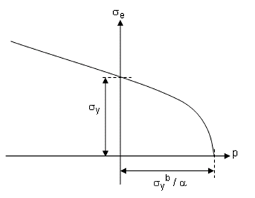
The EDP linear yield criterion form is:

where the user-defined parameters are the pressure sensitivity  and the uniaxial yield stress
  .
.
Defining the EDP Linear Yield Criterion
After initializing the extended Drucker-Prager linear yield criterion (TB ,EDP,,,,LYFUN), enter the following constants (TBDATA):
| Constant | Meaning | Property |
|---|---|---|
| C1 |  | Pressure sensitivity |
| C2 |  | Uniaxial yield stress |
The constants can be defined as a function of temperature
(NTEMP on the TB command),
with temperatures specified for the table entries
(TBTEMP).
The EDP power law yield criteria form is:

where the exponent  , pressure sensitivity
  , and uniaxial yield stress
  are the user-defined parameters.
Defining the EDP Power Law Yield Criterion
After initializing the extended Drucker-Prager power law yield criterion (TB ,EDP,,,,PYFUN), enter the following constants (TBDATA):
| Constant | Meaning | Property |
|---|---|---|
| C1 |  | Pressure sensitivity |
| C2 |  | Exponent |
| C3 |  | Uniaxial yield stress |
The constants can be defined as a function of temperature
(NTEMP on the TB command),
with temperatures specified for the table entries
(TBTEMP).
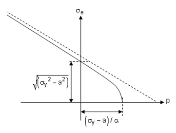
The EDP hyperbolic yield criteria form is:

where the constant  , pressure sensitivity
  , and uniaxial yield stress
  are the user-defined parameters.
In the following figure, the hyperbolic yield criterion is plotted and compared to the linear yield criterion shown in the dashed line:
Defining the EDP Hyperbolic Yield Criterion
After initializing the extended Drucker-Prager hyperbolic yield criterion (TB ,EDP,,,,HYFUN), enter the following constants (TBDATA):
| Constant | Meaning | Property |
|---|---|---|
| C1 |  | Pressure sensitivity |
| C2 |  | Material parameter |
| C3 |  | Uniaxial yield stress |
The constants can be defined as a function of temperature
(NTEMP on the TB command),
with temperatures specified for the table entries
(TBTEMP).
Three EDP flow potentials correspond in form to each of the yield criteria . However, the user-defined parameters for the flow potentials are independent of those for the yield criteria, and any potential can be combined with any yield criterion.
The EDP plastic flow potentials include the following forms:
The linear form of the plastic flow potential is:

where  is the flow potential pressure sensitivity.
Defining the Linear Plastic Flow Potential
After initializing the material data table (TB ,EDP,,,,LFPOT), enter the following constant (TBDATA):
| Constant | Meaning | Property |
|---|---|---|
| C1 |  | Pressure sensitivity |
The material behavior can be defined as a function of temperature
(NTEMP on the TB command),
with temperatures specified for the table entries
(TBTEMP).
The power law form of the plastic flow potential is:

where the exponent  and the pressure sensitivity
  are user-defined parameters.
Defining the Linear Plastic Flow Potential
After initializing the material data table (TB ,EDP,,,,PFPOT), enter the following constants (TBDATA):
| Constant | Meaning | Property |
|---|---|---|
| C1 |  | Pressure sensitivity |
| C2 |  | Exponent |
The material behavior can be defined as a function of temperature
(NTEMP on the TB command),
with temperatures specified for the table entries
(TBTEMP).
The hyperbolic form of the plastic flow potential is:

where the pressure sensitivity  the constant
  are user-defined parameters.
Defining the Linear Plastic Flow Potential
After initializing the material data table (TB ,EDP,,,,HFPOT), enter the following constants (TBDATA):
| Constant | Meaning | Property |
|---|---|---|
| C1 |  | Pressure sensitivity |
| C2 |  | Material parameter |
The material behavior can be defined as a function of temperature
(NTEMP on the TB command),
with temperatures specified for the table entries
(TBTEMP).
The yield stress,  , evolves as a function of the hardening variable,
  :
:

where the hardening variable is the accumulated equivalent plastic strain and is calculated from the summation of:

The plastic strain increment corresponding to each of the plastic flow potentials is:

where  is the deviatoric stress:

The dilatation for each of the flow potentials is:

Associated flow is obtained if the plastic potential form and parameters are set equal to the yield criterion.
The following examples show how to define the EDP material model using various yield criteria and flow potentials:
Example 4.15: EDP -- Linear Yield Criterion and Flow Potential
/prep7
!!! Define linear elasticity constants
mp,ex,1,2.1e4
mp,nuxy,1,0.45
! Extended Drucker-Prager Material Model Definition
! Linear Yield Function
tb,edp,1,1,2,LYFUN
tbdata,1,2.2526,7.894657
! Linear Plastic Flow Potential
tb,edp,1,1,2,LFPOT
tbdata,1,0.566206
Example 4.16: EDP -- Power Law Yield Criterion and Flow Potential
/prep7
!!! Define linear elasticity constants
mp,ex,1,2.1e4
mp,nuxy,1,0.45
! Extended Drucker-Prager Material Model Definition
! Power Law Yield Function
tb,edp,1,1,3,PYFUN
tbdata,1,8.33,1.5
! Power Law Plastic Flow Potential
tb,edp,1,1,2,PFPOT
tbdata,1,8.33,1.5
Example 4.17: EDP -- Hyperbolic Yield Criterion and Flow Potential
/prep7
!!! Define linear elasticity constants
mp,ex,1,2.1e4
mp,nuxy,1,0.45
! Extended Drucker-Prager Material Model Definition
! Hyperbolic Yield Function
tb,edp,1,1,3,HYFUN
tbdata,1,1.0,1.75,7.89
! Hyperbolic Plastic Flow Potential
tb,edp,1,1,2,HFPOT
tbdata,1,1.0,1.75
The EDP Cap material model has a yield criterion similar to the other extended Drucker-Prager yield criteria with the addition of two cap surfaces that truncate the yield surface in tension and compression regions.[ 11 ] The model formulation follows that of Schwer and Murray [ 12 ] and Foster.[ 13 ] The numerical formulation is modified from the work of Pelessone.[ 14 ]
The following topics for the EDP Cap model are available:
The EDP Cap yield criterion is a function of the stress invariants
 ,
,  , and
, and  , given by:

where  is the deviatoric stress.
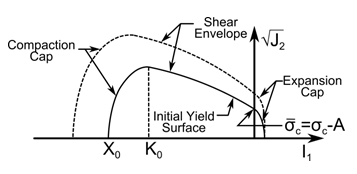
The EDP Cap model uses a closed yield surface comprising three parts:
Expansion cap

Shear envelope

Compaction cap

Figure 4.16: Yield Surface for the Cap Criterion shows the corresponding yield
surface in the meridian  plane. (The plot ignores the dependency of the yield surface
on the stress invariant.)
plane. (The plot ignores the dependency of the yield surface
on the stress invariant.)
The shear envelope function is given by:

where  is the cohesion related yield parameter and is a user defined
material parameter along with
is the cohesion related yield parameter and is a user defined
material parameter along with  ,
,  , and
, and  . This function reduces to the linear Drucker-Prager criterion
for
. This function reduces to the linear Drucker-Prager criterion
for  . For positive values of
  , the shear failure envelope is evaluated at
  = 0, which gives the constant value
  .
.
The compaction cap function is itself a function of the shear envelope function and is given by:

where  is the Heaviside step function,
  is a user-input material parameter, and
  defines the
  value at the intersection of the compaction cap surface with
the shear envelope, given by:
value at the intersection of the compaction cap surface with
the shear envelope, given by:

where  is the user-defined parameter defining the intersection of the
compaction cap with the axis (
is the user-defined parameter defining the intersection of the
compaction cap with the axis ( ):
):
The compaction cap function defines the material yield
surface when  .
.
The expansion cap function is a function of the shear envelope function, given by:
where  is a user-input material parameter. The expansion function
defines the material yield surface when
is a user-input material parameter. The expansion function
defines the material yield surface when  . The expansion cap function intersects with the
axis
. The expansion cap function intersects with the
axis  at
at  .
.
These functions define the yield criterion, given by:
 | (4–33) |
where  is the Lode angle function. The Lode angle is given by:

and the Lode angle function is:

where  is a user-defined material parameter defining the ratio of the
extension strength to compression strength in triaxial loading. To ensure the
convexity of the yield function, the parameter is limited to the range
is a user-defined material parameter defining the ratio of the
extension strength to compression strength in triaxial loading. To ensure the
convexity of the yield function, the parameter is limited to the range
 .
.
Two methods are available to evolve the yield criterion
due to plastic deformation. Hardening or softening of the compaction cap is due
to evolution of  . This value evolves due to plastic volume strain
 , and the relationship is given by [ 15 ]:

where  is the initial value of
  , and the user-defined parameters are
  ,
,  , and
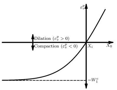
, and  . Shown in Figure 4.17: Relationship Between and , evolution of
includes both hardening and softening depending on the
volumetric plastic strain. Plastic dilation can occur on the shear envelope,
causing the magnitude of to decrease; in this case, to ensure a monotonic relationship
between and , the parameters must satisfy:
. Shown in Figure 4.17: Relationship Between and , evolution of
includes both hardening and softening depending on the
volumetric plastic strain. Plastic dilation can occur on the shear envelope,
causing the magnitude of to decrease; in this case, to ensure a monotonic relationship
between and , the parameters must satisfy:

The EDP Cap model can also be combined with an isotropic hardening model. The isotropic
hardening defines the evolution of the yield surface at the intersection of the
 axis
axis  . The bilinear, multilinear, or nonlinear isotropic hardening
function can be used to define the cohesion-like parameter
. The bilinear, multilinear, or nonlinear isotropic hardening
function can be used to define the cohesion-like parameter  as a function of the equivalent deviatoric plastic
strain.
as a function of the equivalent deviatoric plastic
strain.
The plastic potential used to determine the direction of the plastic strain increment has the same form as the yield criterion given by :
 | (4–34) |
where the potential surface functions are:
 |
 |
 |
and the user-defined potential parameters are  ,
,  ,
,  and
and  .
.
For more information, see Extended Drucker-Prager Cap Model in the Theory Reference.
After initializing the material data table (TB ,EDP,,,,CYFUN), enter the following constants (TBDATA):
| Constant | Meaning | Property | Unit | Range |
|---|---|---|---|---|
| C1 |  | Compaction cap parameter | -- |  |
| C2 |  | Expansion cap parameter | -- |  |
| C3 |  | Compaction cap yield pressure | Force/Length2 |  |
| C4 |  | Cohesion yield parameter | Force/Length2 |  |
| C5 |  | Shear envelope exponent | Length2/Force |  |
| C6 |  | Shear envelope exponential coefficient | Force/Length2 |  |
| C7 |  | Shear envelope linear coefficient | -- |  |
| C8 |  | Ratio of extension to compression strength in triaxial loading | -- |  |
| C9 |  | Limiting value of volumetric plastic strain | -- |  |
| C10 |  | Hardening parameter | Length2/Force | -- |
| C11 |  | Hardening parameter | [Length2/Force]2 | -- |
The yield criterion and hardening behavior can be defined as a function of
temperature (NTEMP on the TB
command), with temperatures specified for the table entries
(TBTEMP).
After initializing the material data table (TB ,EDP,,,,CFPOT), enter the following constants (TBDATA):
| Constant | Meaning | Property | Unit | Range |
|---|---|---|---|---|
| C1 |  | Compaction cap parameter | -- |  |
| C2 |  | Expansion cap parameter | -- |  |
| C3 |  | Shear envelope exponent | Length2/Force |  |
| C4 |  | Shear envelope linear coefficient | -- |  |
The plastic flow potential can be defined as a function of temperature
(NTEMP on the TB command), with
temperatures specified for the table entries (TBTEMP).
If the plastic flow potential is not defined, the yield surface is used as the flow potential, resulting in an associated flow model.
The following example input shows how to define an EDP Cap model by defining the yield criterion, hardening, and plastic flow potential:
Example 4.18: EDP Cap Model Material Constant Input
/prep7
! Define linear elasticity constants
mp,ex  ,1,14e3
mp,nuxy,1,0.0
! Cap yield function
tb,edp ,1,1,,cyfun
tbdata,1,2          ! Rc
tbdata,2,1.5        ! Rt
tbdata,3,-80        ! Xi
tbdata,4,10         ! SIGMA
tbdata,5,0.001      ! B
tbdata,6,2          ! A
tbdata,7,0.05       ! ALPHA
tbdata,8,0.9        ! PSI
! Define hardening for cap-compaction portion
tbdata,9,0.6        ! W1c
tbdata,10,3.0/1000  ! D1c
tbdata,11,0.0       ! D2c
! Cap plastic flow potential function
tb,edp ,1,1,,cfpot
tbdata,1,2          ! RC_bar
tbdata,2,1.5        ! RT_bar
tbdata,3,0.001      ! B_bar
tbdata,4,0.05       ! ALPHA_bar
Use the Gurson model to represent plasticity and damage in ductile porous metals.[ 16 ][ 17 ] When plasticity and damage occur, ductile metal undergoes a process of void growth, nucleation, and coalescence. The model incorporates these microscopic material behaviors into macroscopic plasticity behavior based on changes in the void volume fraction, also known as porosity, and pressure. A porosity increase corresponds to an increase in material damage, resulting in a diminished load-carrying capacity.
The yield criterion and flow potential for the Gurson model is:

where  is the von Mises equivalent stress,
  is the yield stress,
  ,
,  , and
, and  are user-input Tvergaard-Needleman constants, and
  is the modified void volume fraction. The hydrostatic pressure
  is defined as:

The following additional Gurson model topics are available:
For more information, see Gurson's Model in the Theory Reference .
The following figure shows the phenomena of voids at the microscopic scale that are incorporated into the Gurson model:
Figure 4.18: Growth, Nucleation, and Coalescence of Voids at Microscopic Scale
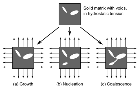
(a): Existing voids grow when the solid matrix is in a hydrostatic-tension state. The solid matrix is assumed to be incompressible in plasticity so that any material volume growth is due to the void volume expansion.
(b): Void nucleation occurs, where new voids are created during plastic deformation due to debonding of the inclusion-matrix or particle-matrix interface, or from the fracture of the inclusions or particles themselves.
(c): Voids coalesce. In this process, the isolated voids establish connections. Although coalescence may not discernibly affect the void volume, the load-carrying capacity of the material begins to decay more rapidly at this stage.
The void volume fraction is the ratio of void volume to the total volume. A volume fraction of 0 indicates no voids and the yield
criterion reduces to the von Mises criterion. A volume fraction of 1 indicates all the material is void. The initial void volume
fraction,  , is a user-defined parameter, and the rate of change of void volume fraction is a combination of the rate of growth
and the rate of nucleation:
, is a user-defined parameter, and the rate of change of void volume fraction is a combination of the rate of growth
and the rate of nucleation:

From the assumption of isochoric plasticity and conservation of mass, the rate of change of void volume fraction due to growth is proportional to the rate of volumetric plastic strain:

Void nucleation is controlled by either the plastic strain or the stress, and is assumed to follow a normal distribution of statistics.
In the case of strain-controlled nucleation, the distribution is described by the mean strain,  , and deviation,
  . The void nucleation rate due to strain control is given by:

where  is the maximum void fraction for nucleated voids,
  is the effective plastic strain, and the rate of effective plastic strain,
  , is determined by equating the microscopic plastic work to the macroscopic plastic work:

In the case of stress-controlled nucleation, void nucleation is determined by the distribution of maximum normal stress on the
interfaces between inclusions and the matrix, equal to  . Stress-controlled nucleation takes into account the effect of triaxial loading on the rate of void nucleation. The
void-nucleation rate for stress control is given by:
. Stress-controlled nucleation takes into account the effect of triaxial loading on the rate of void nucleation. The
void-nucleation rate for stress control is given by:

where distribution of stress is described by the mean stress,  and deviation,
  .
.
The modified void volume fraction,  , is used to model the loss of material load carrying capacity
associated with void coalescence. When the current void volume fraction reaches a
critical value
, is used to model the loss of material load carrying capacity
associated with void coalescence. When the current void volume fraction reaches a
critical value  , the material load carrying capacity decreases rapidly due to
coalescence. When the void volume fraction reaches
, the material load carrying capacity decreases rapidly due to
coalescence. When the void volume fraction reaches  , the load-carrying capacity of the material is lost completely.
The modified void volume fraction is given by:
, the load-carrying capacity of the material is lost completely.
The modified void volume fraction is given by:

The Gurson model can be combined with one of the isotropic hardening models to incorporate isotropic hardening of the yield stress in the Gurson yield criterion.
To combine the Gurson model with Chaboche nonlinear kinematic hardening [ 22 ], the yield criterion is modified to:

where  is the von Mises equivalent modified relative stress, and
  is the effective hydrostatic pressure defined as:

where  is the modified relative stress, which itself is a function of the modified backstress
  :
:


where  is the kinematic hardening backstress.
The rate of effective plastic strain equation is also modified to:

For more information, see Gurson Plasticity with Isotropic/Chaboche Kinematic Hardening in the Theory Reference .
The Gurson material model requires material parameters for the base model combined with parameters for either strain-controlled or stress-controlled nucleation. Additional input is required to define the void coalescence behavior.
To define the Gurson base model, initialize the material data table (TB ,GURSON,,,,BASE), then input the following constants (TBDATA):
| Constant | Meaning | Property |
|---|---|---|
| C1 |  | Initial yield strength |
| C2 |  | Initial porosity |
| C3 |  | First Tvergaard-Needleman constant |
| C4 |  | Second Tvergaard-Needleman constant |
| C5 |  | Third Tvergaard-Needleman constant |
The Gurson base model is combined with either stress- or strain-controlled nucleation.
To define stress-controlled nucleation, initialize the material data table (TB ,GURSON,,,,SSNU), then input the following constants (TBDATA):
| Constant | Meaning | Property |
|---|---|---|
| C1 |  | Nucleation porosity |
| C2 |  | Mean stress |
| C3 |  | Stress standard deviation |
To define strain-controlled nucleation, initialize the material data table (TB ,GURSON,,,,SNNU), then input the following constants (TBDATA):
| Constant | Meaning | Property |
|---|---|---|
| C1 |  | Nucleation porosity |
| C2 |  | Mean strain |
| C3 |  | Strain standard deviation |
Define the void coalescence behavior after defining the Gurson base model and either the stress- or strain-controlled nucleation behavior.
Initialize the material data table (TB ,GURSON,,,,COAL), then input the following constants (TBDATA):
| Constant | Meaning | Property |
|---|---|---|
| C1 |  | Critical porosity |
| C2 |  | Failure porosity |
Following is an example Gurson plasticity material model definition:
Example 4.19: Gurson Model with Isotropic Hardening
/prep7
!!! Define linear elasticity constants
mp,ex,1,207.4E3    ! Young modulus (MPa)
mp,nuxy,1,0.3      ! Poisson's ratio
!!! Define parameters related to Gurson model with
!!! the option of strain-controlled nucleation with
!!! coalescence
f_0=1E-8           ! initial porosity
q1=1.5             ! first Tvergaard constant
q2=1.0             ! second Tvergaard constant
q3=2.25            ! third Tvergaard constant = q1^2
f_c=0.15           ! critical porosity
f_F=0.25           ! failure porosity
f_N=0.04           ! nucleation porosity
s_N=0.1            ! standard deviation of mean strain
strain_N=0.3       ! mean strain
sigma_Y=755        ! initial yielding strength (MPa)
power_N=0.1        ! power value for nonlinear isotropic
                   ! hardening power law
!base model
tb,gurson,1,,5,base
tbdata,1,sigma_Y,f_0,q1,q2,q3
! Strain-controlled nucleation
tb,gurson,1,,3,snnu
tbdata,1,f_N,strain_N,s_N
! Coalescence
tb,gurson,1,,2,coal
tbdata,1,f_c,f_F
! Power law isotropic hardening
tb,nliso,1,,2,POWER
tbdata,1,sigma_Y,power_N
The cast iron plasticity model is used to model gray cast iron. The microstructure of gray cast iron is a two-phase material with graphite flakes embedded in a steel matrix.[ 20 ] The microstructure leads to different behavior in tension and compression. In tension, cracks form due to the graphite flakes and the material is brittle with low strength. In compression, the graphite flakes behave as incompressible media that transmit stress and the steel matrix governs the overall behavior.
The model is isotropic elastic with the same elastic behavior in tension and compression. The yield strength and isotropic hardening behavior may be different in tension and in compression. Different yield criteria and plastic flow potentials are used for tension and compression. It can be combined with Chaboche nonlinear kinematic hardening to simulate cast iron behavior in cyclic loading.
A composite yield surface is used to model different yield behavior in tension and compression. The tension behavior is pressure-dependent and the Rankine maximum stress criterion is used:

where  is the uniaxial tension yield stress. The hydrostatic pressure
 , the von Mises equivalent stress
  , and the Lode angle
  are defined as:


where  and
and  are the stress invariants:

where  is the relative deviatoric stress.
In compression, the pressure-independent von Mises yield criterion is used:

The relative deviatoric stress is:

where  is the nonlinear kinematic backstress given by Equation 4–32 and Equation 4–31 .
The following figure shows the composite yield surface in the meridional plane in which the ordinate and abscissa are von Mises equivalent stress and pressure, respectively:
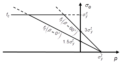
In the following figure, the solid line shows the composite cast iron yield surface in 2D principal stress space:
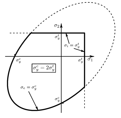
The figure shows that for biaxial loading, the maximum principal stress cannot exceed the tension yield stress. For some combinations of tension and compression loading, the material can yield on either the tension yield surface or the compression yield surface.
As shown in this figure, when the tension and compression yield stress are equal, uniaxial loading yields at the intersection of the compression and tension yield surfaces:
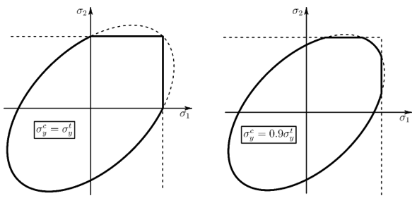
When the tension yield stress is greater than the compression yield stress, uniaxial
loading yields on the compression surface. Because this is not the intended behavior of
the cast iron model, ANSYS, Inc. recommends that the material definition give
 for all states of material evolution.
As shown in the following figure, the tension surface can include a rounding factor,  , to smooth the sharp corners and improve convergence.
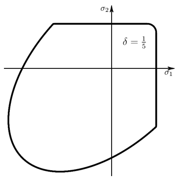
The default is no rounding,  , and the maximum is
  .
.
When a rounding factor is used, the tension yield criterion becomes:

where  and
and  are the ordered principal relative stress values.
The evolution of the yield stress in tension and compression follows the piecewise
user-defined linear stress-strain curves for compression and tension. The tension yield
stress evolves as a function of the equivalent uniaxial plastic strain,  . The evolution of the equivalent uniaxial plastic strain is defined
by equating the uniaxial plastic work increment to the total plastic work increment:
. The evolution of the equivalent uniaxial plastic strain is defined
by equating the uniaxial plastic work increment to the total plastic work increment:

The compression yield stress evolves as a function of the equivalent plastic strain,
 , which is calculated from the increment in plastic strain determined
by consistency with the yield criterion and the flow potential.
, which is calculated from the increment in plastic strain determined
by consistency with the yield criterion and the flow potential.
The plastic flow potential is defined by the von Mises yield criterion in compression and results in an associated flow rule. The flow potential in compression is:

In tension, the Rankine cap yield surface is replaced by an ellipsoidal surface defined by:

where  is a constant function of the user-defined plastic Poisson's ratio,
  :
:

The plastic Poisson's ratio is the absolute value of the ratio of the transverse to
the longitudinal plastic strain under uniaxial tension. It determines the amount of
volumetric expansion during tensile plastic deformation. For  , the tensile flow potential reduces to the von Mises potential. The
tensile flow potential gives a nonassociated flow model and results in an unsymmetric
material stiffness tensor.
, the tensile flow potential reduces to the von Mises potential. The
tensile flow potential gives a nonassociated flow model and results in an unsymmetric
material stiffness tensor.
When the cast iron model is combined with nonlinear kinematic hardening, the backstress is always deviatoric. In tension, only the deviatoric part of the plastic strain is used in the backstress evolution equation.
Define the isotropic elastic behavior (MP or TB ,ELASTIC). Initialize the material data table (TB ,CAST,,,,ISOTROPIC) and input the following constant:
| Constant | Meaning | Property |
|---|---|---|
| C1 |  | Plastic Poisson's ratio |
Enter the tension yield surface rounding factor by initializing the material data table (TB ,CAST,,,,ROUNDING) and input the following constant:
| Constant | Meaning | Property |
|---|---|---|
| C1 |  | Tension yield surface rounding factor |
Enter the tensile multilinear hardening stress-strain points into a data table (TB ,CAST,,,,TENSION). Do the same for the compressive multilinear hardening stress-strain points (TB ,CAST,,,,COMPRESSION). Enter the tension and compression stress-strain points into their respective tables via the TBPT command, with the compression points being entered as positive values:
| Constant | Meaning | Property |
|---|---|---|
| X |  | Plastic strain value |
| Y |  | Stress value |
The plastic Poisson's ratio and stress-strain points can be defined as a function
of temperature (NTEMP value on the TB
command), with individual temperatures specified for the table entries
(TBTEMP).
Example 4.20: Cast Iron
/prep7
mp,  ex, 1,14.773E6
mp,nuxy, 1,0.2273
! Define cast iron model
TB,CAST,1,,,ISOTROPIC
TBDATA,1,0.04
TB,CAST,1,1,5,TENSION
TBPT,,0.000E-00,0.813E+04
TBPT,, 1.13E-04,0.131E+05
TBPT,, 8.69E-04,0.241E+05
TBPT,, 1.55E-03,0.288E+05
TBPT,, 2.32E-03,0.322E+05
TB,CAST,1,1,5,COMPRESSION
TBPT,,0.000E-00,0.300E+05
TBPT,, 1.62E-03,0.500E+05
TBPT,, 4.07E-03,0.581E+05
TBPT,, 6.56E-03,0.656E+05
TBPT,, 9.26E-03,0.700E+05
TB,CHABOCHE,1,1,3,TRATE
TBDATA,1,0,4.0783E3,0.8165
TBDATA,4,3.8973E4,743.0119,3.8973E5,7430.119
Crushable foam materials are cellular solids typically made of metal or polymer. They have a small elastic range followed by nonlinear permanent deformation governed by buckling and deformation in the cell walls and struts. Common applications include packaging materials such as expanded polystyrene where energy absorption is important, and foam-core sandwich panels where a high stiffness-to-weight ratio is required.
Based on the initial work of Desphande and Fleck , the model captures the monotonic yielding, hardening evolution, and elastic unloading of crushable foam materials. It is likely unsuitable for high-rate loading, large deformations, or non-monotonic yield behavior such as cyclic loading.
The yield behavior of crushable foams depends on both the deviatoric and hydrostatic loading. Shown in Figure 4.23: Crushable Foam Yield Surface , the yield function is:

where  and
and  are the evolving uniaxial and absolute hydrostatic compression yield values, and the von Mises effective stress and
hydrostatic pressure are:
are the evolving uniaxial and absolute hydrostatic compression yield values, and the von Mises effective stress and
hydrostatic pressure are:

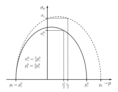
The derived material parameters are the shape factor  , the hydrostatic center of the yield surface
  , and the maximum shear
  . They are derived from the input parameters for initial uniaxial yield stress
  , initial absolute hydrostatic compression yield stress
  , and hydrostatic tension yield stress
  . Defining the yield stress ratios,

the derived material parameters are given by:

The uniaxial yield stress  evolves as a function of the equivalent plastic strain
  :
:

where  is a user-defined multilinear hardening function.
The yield surface hardens in such a manner that both the hydrostatic tension yield  and the aspect ratio of the yield surface ellipse
  are constant during the hardening of
  . This evolution gives the hardening of absolute hydrostatic compression yield as a function of the uniaxial yield
stress hardening:
. This evolution gives the hardening of absolute hydrostatic compression yield as a function of the uniaxial yield
stress hardening:

The evolution of the plastic equivalent strain  follows one of two methods that you select. The evolution is based on the work-rate conjugate to either the flow potential or the uniaxial yield stress :

where  is the plastic strain rate and
  is the flow potential:

where  is a shape factor that is a function of the plastic Poisson’s ratio
  , as follows:

This non-associated flow potential results in an unsymmetric material stiffness matrix.
Define the isotropic or anisotropic elastic behavior (MP or TB ,ELASTIC). Initialize the crushable foam yield data table (TB ,CFOAM,,,,YIELD) and input the following constants:
| Constant | Meaning | Property |
|---|---|---|
| C1 |  | Initial uniaxial compression yield |
| C2 |  | Initial hydrostatic compression yield |
| C3 |  | Hydrostatic tension yield |
The yield stress values must satisfy  , ,  , ,  , and , and  . . |
To define the hardening of the uniaxial compressive yield, initialize a multilinear hardening data table (TB ,CFOAM,,,,MHARD) and define the following data pairs:
| Constant | Meaning | Property |
|---|---|---|
| X |  | Plastic strain value |
| Y |  | Relative stress value |
At  , the relative stress value should start at , the relative stress value should start at  and increase monotonically. (Decreasing values of relative stress give softening material behavior and may lead
to convergence difficulty.) and increase monotonically. (Decreasing values of relative stress give softening material behavior and may lead
to convergence difficulty.) |
The hardening type is specified via a data table (TB ,CFOAM,,,,HTYPE) with the following input:
| C1 = 0 (default) specifies that the equivalent plastic strain evolves based on work conjugate to the plastic potential. C1 = 1 specifies that the equivalent plastic strain evolves based on work conjugate to the uniaxial compressive yield stress. |
The shape of the plastic potential is determined by the plastic Poisson’s ratio, entered in a data table (TB ,CFOAM,,,,PPR) with the following input:
| Constant | Meaning | Property |
|---|---|---|
| C1 |  | Plastic Poisson’s ratio |
The valid range for the plastic Poisson's ratio is  . . |
Example 4.21: Defining the Crushable Foam Material Model
/prep7
mp,  ex, 1,3e6
mp,nuxy, 1,0.2
p_c0 = 1e6
sigma_c0 = 5/4*p_c0
p_t0 = 4/5*p_c0
nu_p = 0.05
hardening_flag = 1
! yield stresses
TB,CFOAM,1,,,YIELD
TBDATA,1, sigma_c0, p_c0, p_t0
! plastic Poisson's ratio
TB,CFOAM,1,,,PPR
TBDATA,1, nu_p
! hardening type
TB,CFOAM,1,,,HTYPE
TBDATA,1, hardening_flagst
! hardening curve
TB,CFOAM,1,1,,MHARD
TBPT,,0.0, 1.0
TBPT,,0.5, 2.2
TBPT,,1  , 2.9
TBPT,,1.5, 3.0
TBPT,,2  , 3.1
Sintering coalesces a powdered material into a solid or porous mass using heat (and typically densification) without introducing liquefaction. In an additive manufacturing analysis, you can model metal powders in a green state undergoing a sintering process. The green state may have been produced via a binder jetting process, a metal injection molding (MIM) process, or by some other means.
Given a specified temperature cycle and the initial state variables for the underlying powder material (initial relative density, initial particle size, and optionally the initial grain size), the sintering model simulates the densification and viscous shear response of the material under any external load (such as gravity).
Note: The remaining content of this section is accessible for licensed users with Ansys credentials. If you already have an Ansys account, log in by clicking CUSTOMER LOGIN in the upper right corner of the help page. If not, contact your Ansys support provider to learn about license options.