


Use thermal-diffusion analysis to perform coupled thermal-diffusion analyses with temperature-dependent material properties. Applications include moisture migration in electronics packages. You can also use this capability to perform a thermomigration analysis; applications include thermophoresis and thermomigration of atoms and vacancies in solder joints.
For theoretical background, see Thermal-Diffusion Coupling in the Theory Reference.
The following related topics are available:
The program includes a variety of elements that you can use to perform a coupled thermal-diffusion analysis. Table 2.32: Elements Used in Thermal-Diffusion Analyses summarizes these elements. For detailed descriptions of the elements and their characteristics (degrees of freedom, KEYOPT options, inputs and outputs, etc.), see the Element Reference.
For a coupled thermal-diffusion analysis, you need to select the TEMP and CONC element degrees of freedom by setting KEYOPT(1) to 100010 with PLANE222, PLANE223, SOLID225, SOLID226, or SOLID227.
Table 2.32: Elements Used in Thermal-Diffusion Analyses
| Elements | Effects | Analysis Types |
|---|---|---|
|
PLANE222 - 4-Node Coupled-Field Quadrilateral PLANE223 - 8-Node Coupled-Field Quadrilateral SOLID225 - 8-Node Coupled-Field Hexahedral SOLID226 - 20-Node Coupled-Field Hexahedral SOLID227 - 10-Node Coupled-Field Tetrahedral |
Temperature-dependent material properties, including temperature-dependent saturated concentration (CSAT) Thermomigration |
Static Full Transient |
To perform a thermal-diffusion analysis:
Select a coupled-field element that is appropriate for the analysis (Table 2.32: Elements Used in Thermal-Diffusion Analyses). Use KEYOPT(1) to select the TEMP and CONC element degrees of freedom.
Specify thermal material properties:
Specify diffusion material properties:
Specify diffusivity (DXX, DYY, DZZ) (MP).
If working with normalized concentration, specify saturated concentration (CSAT) (MP). For more information, see Normalized Concentration Approach in the Theory Reference.
To account for the thermal transport (thermomigration) effect:
Specify the heat of transport/Boltzmann constant ratio (Q/k) using constant C3 (TBDATA) for the migration table, TB,MIGR. Alternatively, you can specify the molar heat of transport/universal gas constant ratio (Q/R) using the same format. For more information, see Migration Model in the Material Reference.
If the diffusivity coefficients depends on temperature as shown in Equation 5–7 of Migration Model in the Material Reference:
Apply thermal and diffusion loads, initial conditions, and boundary conditions:
Thermal loads, initial conditions, and boundary conditions include temperature (TEMP), heat flow rate (HEAT), convection (CONV), heat flux (HFLUX), radiation (RDSF), and heat generation (HGEN).
Specify temperature offset from absolute zero to zero (TOFFST).
Diffusion loads, initial conditions, and boundary conditions include concentration (CONC), diffusion flow rate "force" (RATE), diffusion flux (DFLUX), and diffusing substance generation rate (DGEN).
Specify analysis type and solve:
Analysis type can be static or full transient.
You can use KEYOPT(2) to select a strong (matrix) or weak (load vector) thermal-diffusion coupling. Strong coupling produces an unsymmetric matrix. Weak coupling produces a symmetric matrix, but requires more iterations to achieve a coupled response.
Set convergence values (CNVTOL) with:
Temperature (TEMP) and heat flow (HEAT) labels
Concentration (CONC) and diffusion flow rate (RATE) labels
For problems having convergence difficulties, activate the line-search capability (LNSRCH).
Post-process thermal and diffusion results:
Thermal results include temperature (TEMP), thermal gradient (TG), and thermal flux (TF).
Diffusion results include concentration (CONC), concentration gradient (CG), and diffusion flux (DF).
The effect of film coefficient and air temperature on convective drying of a potato slice is demonstrated. A detailed model description can be found in “Inverse Approaches to Drying of Sliced Foods” by G. H. Kanevce, L. P. Kanevce, V. B. Mitrevski, and G. S. Dulikravich. Inverse Problems, Design and Optimization Symposium, Miami: April 16-18, 2007.
The following topics are available:
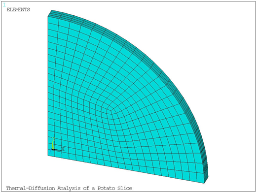
A quarter symmetry model of a potato slice with thickness h = 3 mm and radius r = 40 mm (Figure 2.94: Finite Element Model of the Potato Slice) is modeled using the diffusion-thermal analysis option (KEYOPT(1)=100010) of SOLID226. The potato has initial normalized concentration conc0 = 1 and initial temperature temp0 = 20 °C.
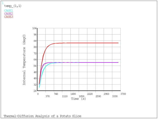
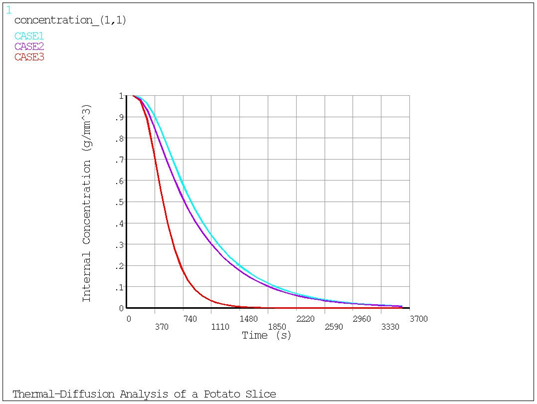
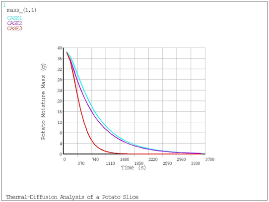
Three transient thermal-diffusion analyses with run times t = 3600 s are performed on the potato slice to determine the effect of film coefficient and bulk temperature on drying. The outer surfaces of the potato are subjected to a convection surface load and an applied normalized concentration conc1 = 0. The concentration load simulates dry surrounding conditions.
The first analysis is performed with film coefficient h1 = 3.2e-5 W/mm2 °C and bulk temperature temp1 = 60 °C.
The second analysis is performed with film coefficient h2 = 5.9e-5 W/mm2 °C and bulk temperature temp1 = 60 °C.
The third analysis is performed with film coefficient h1 = 3.2e-5 W/mm2 °C and bulk temperature temp2 = 85 °C.
Table 2.33: Problem Specifications
| Material Properties | Geometric Properties | Loading | ||||||||||||||||||||||
|---|---|---|---|---|---|---|---|---|---|---|---|---|---|---|---|---|---|---|---|---|---|---|---|---|
|
Thermal Conductivity:
Mass Density:
Specific Heat:
Saturated Concentration:
Diffusivity Coefficient versus Temperature:
|
Radius: r = 40 mm Thickness: h = 3 mm |
Initial Concentration:
Initial Temperature:
Applied Concentration:
First Analysis: Bulk Temperature:
Film Coefficient:
Second Analysis: Bulk Temperature: temp1 = 60 °C Film Coefficient:
Third Analysis: Bulk Temperature:
Film Coefficient:
|
The node located at the center of the potato slice was used for postprocessing. The results indicate that increasing the film coefficient increases the drying rate of the potato slice. Likewise, increasing the air temperature also increases the drying rate.
/title, Thermal-Diffusion Analysis of a Potato Slice

! *** Potato dimensions
r=40					! Radius, mm
h=3					! Thickness, mm

! *** Material properties of potato
! *** Thermal properties assumed constant
k=4e-4				! Thermal conductivity, W/mm/K
p=7.55e-4				! Mass density, g/mm^3
c=4.34			 	! Specific heat, J/g/degC
csat=3.62e-3			! Saturated concentration, g/mm^3
! Temperatures for diffusivity coefficients, degC
t1=10 $t2=20 $t3=30 $t4=40 $t5=50 $t6=60 $t7=70 $t8=80 $t9=90
! Diffusivity coefficients, mm^2/s
d1=8.97e-5 $d2=1.68e-4 $d3=3.00e-4 $d4=5.18e-4 $d5=8.66e-4	$d6=1.40e-3 $d7=2.20e-3 $d8=3.38e-3 $d9=5.07e-3

! *** Loads
temp0=20				! Initial potato temperature, degC
temp1=60				! Bulk temp. for CASE1 and CASE2, degC
temp2=85				! Bulk temperature for CASE3, degC
conc0=1				! Initial normalized concentration
conc1=0				! Applied normalized concentration
h1=3.2e-5				! Film coefficient for CASE1 and CASE3, W/mm^2/degC
h2=5.9e-5				! Film coefficient for CASE2, W/mm^2/degC

t=3600				! Time, s
sub=40 				! Number of substeps

/PREP7
et,1,226,100010 			! Thermal-diffusion solid
keyopt,1,10,1			! Diagonalized damping matrix
mshmid,2				! No midside nodes
mp,kxx,1,k
mp,dens,1,p
mp,csat,1,csat
mp,c,1,c
mptemp,1,t1,t2,t3,t4,t5,t6
mptemp,,t7,t8,t9
mpdata,dxx,1,1,d1,d2,d3,d4,d5,d6
mpdata,dxx,1,,d7,d8,d9
cylind,0,r,0,h,0,90
esize,3
lesize,9,0.75
vmesh,all

! *** Components and nodes for loads and postprocessing
asel,s,area,,3
nsla,,1
nsel,a,loc,z,0
nsel,a,loc,z,h
cm,OUTERSURFACE,node		! Nodes at outer surface
nsel,s,loc,x,0
nsel,r,loc,y,0
nsel,r,loc,z,h/2
*get,CENTER,node,,num,min	! Node at center

! *** Loads and boundary conditions
cmsel,s,OUTERSURFACE
sf,all,conv,h1,temp1		! Convection surface load, CASE1
d,all,conc,conc1			! Applied concentration
alls
ic,all,conc,conc0		! Initial conditions
ic,all,temp,temp0
fini

/SOLU
antype,trans
outres,all,all
kbc,1					! Stepped load
time,t
nsubs,sub
cnvtol,temp,1,1e-7
cnvtol,conc,1,1e-7
solve
fini

/POST1
*dim,concentration_,table,sub,3
*dim,mass_,table,sub,3
*dim,temp_,table,sub,3
*do,ii,1,sub
  set,1,ii
  *get,time_ii,active,,set,time
  concentration_(ii,0)=time_ii    	! Time, s
  mass_(ii,0)=time_ii
  temp_(ii,0)=time_ii
  *get,center_conc,node,CENTER,conc
  concentration_(ii,1)=center_conc	! Normalized concent., CASE1
  *get,center_temp,node,CENTER,temp
  temp_(ii,1)=center_temp  	! Temperature, degC, CASE1
  etable,conc,smisc,1
  etable,volu,volu
  smult,watr,conc,volu
  ssum
  *get,moisture,ssum,,item,watr
  mass_(ii,1)=moisture*4	! Moisture mass of entire slice, g, CASE1
*enddo
fini

/PREP7
! *** Loads
cmsel,s,OUTERSURFACE
sf,all,conv,h2,temp1		! Convection surface load, CASE2
alls
ic,all,conc,conc0		! Initial conditions
ic,all,temp,temp0
fini

/SOLU
antype,trans
outres,all,all
kbc,1					! Stepped load
time,t
nsubs,sub
cnvtol,temp,1,1e-7
cnvtol,conc,1,1e-7
solve
fini

/POST1
*do,ii,1,sub
  set,1,ii
  *get,time_ii,active,,set,time
  *get,center_conc,node,CENTER,conc
  concentration_(ii,2)=center_conc	! Normalized concent., CASE2
  *get,center_temp,node,CENTER,temp
  temp_(ii,2)=center_temp  ! Temperature, degC, CASE2
  etable,conc,smisc,1
  etable,volu,volu
  smult,watr,conc,volu
  ssum
  *get,moisture,ssum,,item,watr
  mass_(ii,2)=moisture*4	! Moisture mass of entire slice, g, CASE2
*enddo
fini

/PREP7
! *** Loads
cmsel,s,OUTERSURFACE
sf,all,conv,h1,temp2		! Convection surface load, CASE3
alls
ic,all,conc,conc0		! Initial conditions
ic,all,temp,temp0
fini

/SOLU
antype,trans
outres,all,all
kbc,1					! Stepped load
time,t
nsubs,sub
cnvtol,temp,1,1e-7
cnvtol,conc,1,1e-7
solve
fini

/POST1
*do,ii,1,sub
  set,1,ii
  *get,time_ii,active,,set,time
  *get,center_conc,node,CENTER,conc
  concentration_(ii,3)=center_conc	! Normalized concent., CASE3
  *get,center_temp,node,CENTER,temp
  temp_(ii,3)=center_temp  	! Temperature, degC, CASE3
  etable,conc,smisc,1
  etable,volu,volu
  smult,watr,conc,volu
  ssum
  *get,moisture,ssum,,item,watr
  mass_(ii,3)=moisture*4	! Moisture mass of entire slice, g, CASE3
*enddo

/axlab,x,Time (s)
/xrange,,t+100
/gcolu,1,CASE1
/gcolu,2,CASE2
/gcolu,3,CASE3
/axlab,y,Internal Temperature (degC)
*vplot,temp_(1,0),temp_(1,1),2,3
/axlab,y,Internal Concentration (g/mm^3)
*vplot,concentration_(1,0),concentration_(1,1),2,3
/axlab,y,Potato Moisture Mass (g)
*vplot,mass_(1,0),mass_(1,1),2,3
fini