


Building a finite element model requires more of your time than any other part of the analysis. First, you specify a jobname and analysis title. Then, you use the PREP7 preprocessor to define the element types, element real constants, material properties, and the model geometry.
A jobname is not required for an analysis but is recommended.
The jobname is a name that identifies an analysis job. When you define a jobname for an analysis, the jobname becomes the first part of the name of all files the analysis creates. (The extension or suffix for these files' names is a file identifier such as .db.) Assigning a jobname for each analysis ensures that no files are overwritten.
If no jobname is specified, all files are named FILE. You can change the default jobname by using the initial jobname entry option when you start the Mechanical APDL program (via the launcher or execution command) or via the /FILNAME command.
The /FILNAME command is valid only at the Begin level. It
lets you change the jobname even if you had specified an initial jobname after
starting the program. The jobname applies only to files you open after using
/FILNAME and not to files that were already open. To
start new files (such as the log file, Jobname.log, and
error file Jobname.err) via /FILNAME,
set the Key argument to 1; otherwise, the files that
were already open will still have the initial jobname.
The /TITLE command defines a title for the analysis. The program includes the title on all graphics displays and on the solution output. Issue the /STITLE command to add subtitles, which appear in the output but not in graphic displays.
The program does not assume a system of units for your analysis. Except in magnetic field analyses, you can use any system of units so long as you make sure that you use that system for all the data you enter. (Units must be consistent for all input data.)
For micro-electromechanical systems (MEMS), where dimensions are on the order of microns, see the conversion factors in System of Units in the Coupled-Field Analysis Guide.
Using the /UNITS command, you can set a marker in the database indicating the system of units that you are using. This command does not convert data from one system of units to another; it simply serves as a record for subsequent reviews of the analysis.
The element library offers many element types. Each element type has a prefix identifying the element category and a unique ID number: PLANE182, SOLID185, BEAM188, ELBOW290, and so on.
The element type determines:
The degree-of-freedom set (which in turn implies the discipline - structural, thermal, magnetic, electric, quadrilateral, brick, etc.)
Whether the element lies in 2D or 3D space.
BEAM188, for example, has six structural degrees of freedom (UX, UY, UZ, ROTX, ROTY, ROTZ), is a line element, and can be modeled in 3D space. PLANE77 has a thermal degree of freedom (TEMP), is an 8-node quadrilateral element, and can be modeled only in 2D space.
You must be in PREP7, the general preprocessor, to define element types. To do so, use the ET family of commands (ET, ETCHG, etc.). Define the element type by name and give the element a type reference number.
This table of type reference number versus element name is called the element type table. While defining the actual elements, point to the appropriate type reference number via the TYPE command.
If you are building a model using beams or shells, issue the section commands (SECTYPE, SECDATA, etc.) to define and use cross sections in your models. See Beam and Pipe Cross Sections in the Structural Analysis Guide for information about using BeamTool to create cross sections.
For line and area elements that require geometry data (cross-sectional area, thickness, diameter, etc.) to be specified as sections, you can verify the input graphically via the /ESHAPE and EPLOT commands (in that order).
The program displays the elements as solid elements, determining the geometry from the section shape and dimension. A rectangular cross-section is used for links.
Element real constants are properties that depend on the element type, such as contact stiffness and penetration. Not all element types require real constants, and different elements of the same type may have different real constant values.
Specify real constants via the R family of commands (R, RMODIF, etc.) or their equivalent menu paths; see the Command Reference for further information. As with element types, each set of real constants has a reference number, and the table of reference number versus real constant set is called the real constant table. While defining the elements, point to the appropriate real constant reference number via the REAL command.
Following are hints for defining real constants:
For models using multiple element types, use a separate real constant set (that is, a different REAL reference number) for each element type. The program issues a warning message if multiple element types reference the same real constant set. However, a single element type may reference several real constant sets.
To verify your real constant input, issue the RLIST and ELIST commands, with
RKEY= 1. RLIST lists real constant values for all sets. The command ELIST,,,,,1 displays an easier-to-read list that shows, for each element, the real constant labels and their values.
Most element types require material properties. Depending on the application, material properties can be linear (see Linear Material Properties) or nonlinear (see Nonlinear Material Properties).
As with element types and real constants, each set of material properties has a material reference number. The table of material reference numbers versus material property sets is called the material table. Within one analysis, you may have multiple material property sets (to correspond with multiple materials used in the model). The program identifies each set with a unique reference number.
While defining the elements, point to the appropriate material reference number via MAT.
See Material Properties for more information about the types of material properties and how to define them.
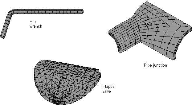
Once you have defined material properties, the next step in an analysis is generating a finite element model - nodes and elements - that adequately describes the model geometry. The graphic below shows some sample finite element models:
There are two methods to create the finite element model: solid modeling and direct generation. With solid modeling, you describe the geometric shape of your model, then instruct the program to automatically mesh the geometry with nodes and elements. You can control the size and shape in the elements that the program creates. With direct generation, you "manually" define the location of each node and the connectivity of each element. Several convenience operations, such as copying patterns of existing nodes and elements, symmetry reflection, etc. are available.
Details of the two methods and many other aspects related to model generation - coordinate systems, working planes, coupling, constraint equations, etc. - are described in the Modeling and Meshing Guide.