The following complete analysis examples, including command input, are presented here:
For additional examples of a rotating structure analysis using a rotating reference frame, see the following test cases in the Mechanical APDL Verification Manual:
See also:
The following example presents a Campbell diagram analysis of a Jeffcott rotor, first in a stationary reference frame (SRF) and then in a rotating reference frame (RRF). It demonstrates the relationship between RRF and SRF frequencies.
The model is a massless rigid rotating shaft supported at its ends by identical bearings (COMBI214). A disk is mounted on the shaft and modelled with a point mass element (MASS21) located at 0.2 m from its end. The shaft is modeled using constraint equations (CERIG command). The rotational velocity varies between 0 rpm and 10,000 rpm along the Z axis.

Inertia properties of the mass:
| Mass = 25 kg |
| Inertia (XX,YY) = 5 kg·m2 |
| Inertia (ZZ) = 10 kg·m2 |
Shaft length: 1 m
Bearing stiffness: 4e+6 N/m
/title, Campbell Diagram Analysis of Jeffcott Rotor

! ** parameters

mass = 25
iz = 10
ix = 5
iy = 5
k = 4e+6
pi = acos(-1)
ratio = pi/30
omend = ratio*10000

/prep7

n,1,0,0,0
n,2,0,0,1
n,3,0,0,0.2

et,1,mass21		! fake mass for CERIG 6 DOFs
r,1
type,1
real,1
e,1
e,2

et,2,mass21
r,2,mass,mass,mass,ix,iy,iz
type,2
real,2
e,3

cerig,3,all,all

n,100,,,0
n,110,,,1

et,3,combi214           ! bearing
r,3,k,k
type,3
real,3
e,100,1
e,110,2

d,all,uz,0
d,all,rotz,0
d,100,all,0
d,110,all,0
finish

! *** Multistep modal analysis in SRF

nbp2 = 10
domg2 = omend/nbp2
*dim,omg2,array,nbp2+1
*do,iloop,1,nbp2
 omg2(iloop+1) = omg2(iloop) + domg2
*enddo
omg2(1) = domg2*1e-2

/solu
antype,modal
modopt,damp,8
mxpand,8
coriolis,on,,,on
*do,iloop,1,nbp2+1
   omega,,,omg2(iloop)
   solve
*enddo
finish

! ** Campbell in SRF

/post1
/show,png,rev
/yrange,0,400
plcamp,,1,rpm
prcamp,,1,rpm
/show,close
*dim,FRQ_SRF,ARRAY,4
*do,iloop,1,4
   *get,FRQ_SRF(iloop),CAMP,iloop,FREQ,nbp2+1
*enddo
finish


! *** Multistep modal analysis in RRF

nbp = 20
domg = omend/nbp
*dim,omg,array,nbp+1
*do,iloop,1,nbp
 omg(iloop+1) = omg(iloop) + domg
*enddo
omg(1) = domg*1e-2

/solu
antype,modal
modopt,damp,8
mxpand,8
coriolis,on
*do,iloop,1,nbp+1
   omega,,,omg(iloop)
   solve
*enddo
finish

! ** Campbell diagram in RRF

/post1
/show,png,rev
/yrange,0,280
/gthk,curve,-1         ! no curve - only markers
/psymb,mark,4          ! marker size
*do,iloop,1,6
 /gmarker,iloop,3      ! marker type
*enddo
plcamp,,,rpm
prcamp,,,rpm
/show,close
*dim,FRQ_RRF,ARRAY,4
*do,iloop,1,4
   *get,FRQ_RRF(iloop),CAMP,iloop,FREQ,nbp+1
*enddo
finish

! ** Compare SRF and RRF frequencies at maximum spin
frend = omend/(2*pi)
*dim,FRQ_SRF_INRRF,ARRAY,4
FRQ_SRF_INRRF(1) = abs(FRQ_SRF(2) - frend)
FRQ_SRF_INRRF(2) = FRQ_SRF(1) + frend
FRQ_SRF_INRRF(3) = abs(FRQ_SRF(4) - frend)
FRQ_SRF_INRRF(4) = FRQ_SRF(3) + frend
*status,FRQ_SRF
*status,FRQ_RRF
*status,FRQ_SRF_INRRF
The outputs for this analysis are shown in the figures below.
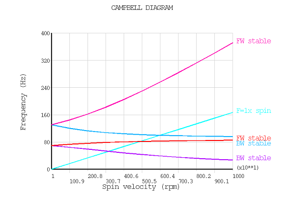
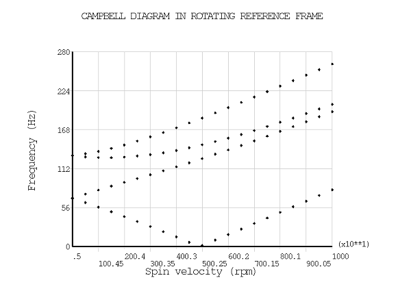
Figure 5.3: Relationship Between SRF and RRF Frequencies
PARAMETER STATUS- FRQ_SRF  (     21 PARAMETERS DEFINED)
                  (INCLUDING        2 INTERNAL PARAMETERS)

      LOCATION                VALUE
        1       1       1    27.1023115
        2       1       1    85.1999476
        3       1       1    95.8462296
        4       1       1    371.081927

 PARAMETER STATUS- FRQ_RRF  (     21 PARAMETERS DEFINED)
                  (INCLUDING        2 INTERNAL PARAMETERS)

      LOCATION                VALUE
        1       1       1    81.4667190
        2       1       1    193.768978
        3       1       1    204.415260
        4       1       1    262.512896

 PARAMETER STATUS- FRQ_SRF_INRRF  (     21 PARAMETERS DEFINED)
                  (INCLUDING        2 INTERNAL PARAMETERS)

      LOCATION                VALUE
        1       1       1    81.4667190
        2       1       1    193.768978
        3       1       1    204.415260
        4       1       1    262.512896
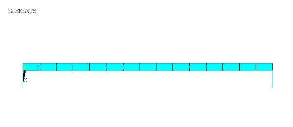
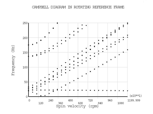
The following example from the reference [Friswell et al.] shows a Campbell diagram analysis in the rotating reference frame of an asymmetric rotor carrying two disks, as shown in Figure 5.4: Asymmetric Rotor.
The model is an asymmetric shaft (BEAM188) defined by its cross-section and inertias supported at its ends by identical bearings (COMBI214). The disks are modeled with two point-mass elements (MASS21) located at 0.5 m and 1 m.
The undamped system is studied first, then damping is introduced in the bearings.
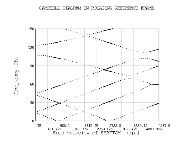
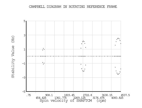
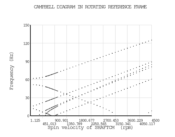
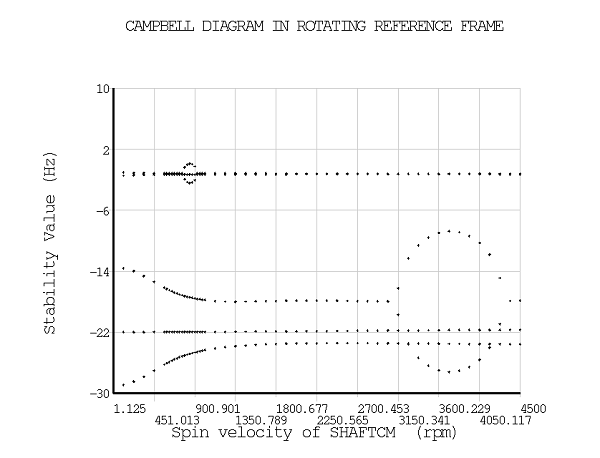
The rotational velocity varies between 0 rpm and 4500 rpm. The evolution of the frequencies and of the stability values are plotted for both undamped and damped systems (PLCAMP). To obtain a more precise shape of the curves around the instability regions, more points are requested by specifying a smaller rotational velocity increment.
Only the shaft and disks are rotating, and the bearings are stationary. Bearing
damping thus introduces rotating damping terms in the rotating reference frame
analysis (RotDamp = ON on the CORIOLIS
command).
Friswell, M., Penny, J., Garvey, S., and Lees, A. Dynamics of Rotating Machines. Cambridge University Press. 2010.
Geometric properties of the shaft:
| Length = 1.5 m |
| Cross sectional area = 2e-3 m2 |
| Moments of area (Iax, Iay) = (4.2043e-7 m4, 2.4112e-7 m4) |
Geometric properties of the disk:
| Diameter_1 = 0.28 m |
| Thickness_1 = 0.07 m |
| Diameter_2 = 0.07 m |
| Thickness_2 = 0.35 m |
Material properties:
| Young’s modulus (E) = 2.11e+11 N/m2 |
| Density = 7810 kg/m3 |
| Poisson's ratio (ν) = 0.3 |
Bearing properties:
| Stiffness (K) = 1e+6 N/m |
| Damping (C) = 5e+3 N·s/m |
/title, Campbell of Non-Axisymmetric Beam Model


! *** parameters

l = 1.5
a = 2e-3
iax = 4.2043e-7
iay = 2.4112e-7
jdummy = 1e-7

e = 211e+9
dens = 7810
nu = 0.3

lld = 0.5
lrd = 1

thkld = 0.07
dld = 0.28

thkrd = 0.07
drd = 0.35

k = 1e+6
c = 5e+3

pi = acos(-1)
ratio = pi/30
omend = 4500

esiz = 0.1

rld = dld/2
mld = pi*thkld*dens*rld**2
idld = mld*(3*rld**2 + thkld**2)/12
ipld = mld*rld**2/2

rrd = drd/2
mrd = pi*thkrd*dens*rrd**2
idrd = mrd*(3*rrd**2 + thkrd**2)/12
iprd = mrd*rrd**2/2

/prep7

! *** geometry

k,1
k,2,,,lld
k,3,,,lrd
k,4,,,l

l,1,2
l,2,3
l,3,4

! *** mesh

lesize,all,esiz

et,1,beam188
mp,ex,1,e
mp,dens,1,dens
mp,nuxy,1,nu
sectype,1,beam,asec
secdata,a,iax,,iay,,jdummy
type,1
mat,1
secnum,1
lmesh,1,3

et,2,mass21
r,2,mld,mld,mld,idld,idld,ipld
type,2
real,2
e,node(0,0,lld)

et,3,mass21
r,3,mrd,mrd,mrd,idrd,idrd,iprd
type,3
real,3
e,node(0,0,lrd)

et,4,combi214
r,4,k,k
type,4
real,4
n,100,0.1
n,104,0.1,,l
e,100,node(0,0,0)
e,104,node(0,0,l)

! *** boundary conditions

d,all,rotz
d,all,uz
d,100,all
d,104,all

! *** component definition

esel,,type,,1,3
cm,shaftcm,elem
allsel
finish

save,case1,db

! *************** Campbell diagram analysis of undamped model

nbp = 60
domg = omend/nbp
nbspins = 73
*dim,omg,array,nbspins+1
*do,iloop,1,nbspins
 *if,omg(iloop)+domg,gt,675,and,omg(iloop)+domg,lt,1000,then,
    omg(iloop+1) = omg(iloop) + domg/2
 *elseif,omg(iloop)+domg,gt,2550,and,omg(iloop)+domg,lt,2925,then,
    omg(iloop+1) = omg(iloop) + domg/2
 *elseif,omg(iloop)+domg,gt,4200,then,
    omg(iloop+1) = omg(iloop) + domg/2
 *else
    omg(iloop+1) = omg(iloop) + domg
 *endif
*enddo
omg(1) = domg*1e-2

/solu
antype,modal
modopt,damp,20
mxpand,20
coriolis,on
*do,iloop,1,nbspins+1
   cmomega,shaftcm,,,omg(iloop)*ratio
   solve
*enddo
finish

/post1
/show,png,rev
/yrange,0,150
/gthk,curve,-1
/psymb,mark,2
*do,iloop,1,10
 /gmarker,iloop,3
*enddo
plcamp,,,rpm,,shaftcm,,yes,yes
prcamp,,,rpm,,shaftcm,,yes,yes
/yrange,-5,5
plcamp,,,rpm,,shaftcm,1,yes,yes
prcamp,,0,rpm,,shaftcm,1,yes,yes
/show,close
finish

/clear,nostart

! ***************** Campbell diagram analysis of damped model

/filname,case2
resume,case1,db

/prep7
rmodif,4,5,C,C   ! add damping in bearing
finish

nbp2 = 40
nbp = 52
domg = omend/nbp2
*dim,omg,array,nbp+1
*do,iloop,1,nbp
  *if,omg(iloop)+domg,gt,600,and,omg(iloop)+domg,lt,1100,then,
     omg(iloop+1) = omg(iloop) + domg/4
 *else
     omg(iloop+1) = omg(iloop) + domg
 *endif
*enddo
omg(1) = domg*1e-2

/solu
antype,modal
modopt,damp,15
mxpand,15
coriolis,on,,,,on     ! activate rotating damping effect
*do,iloop,1,nbp+1
   cmomega,shaftcm,,,omg(iloop)*ratio
   solve
*enddo
finish

/post1
/show,png,rev
/yrange,0,150
/gthk,curve,-1
/psymb,mark,2
*do,iloop,1,10
 /gmarker,iloop,3
*enddo
plcamp,,,rpm,,shaftcm,,yes,yes
prcamp,,,rpm,,shaftcm,,yes,yes
/yrange,-30,10
plcamp,,,rpm,,shaftcm,1,yes,yes
prcamp,,0,rpm,,shaftcm,1,yes,yes
/show,close
finish
Without damping, instability regions are identified based on the sign of the stability value. The stability of the rotor is improved when damping is introduced. The results are shown in the graphs below.
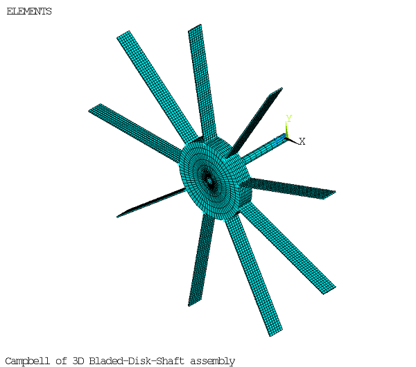
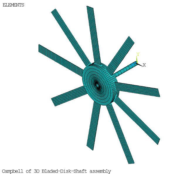
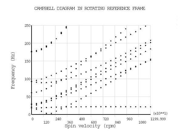
The following example from the reference [Ruffini et al.] presents a Campbell analysis of the 3D bladed shaft-disk assembly shown in Figure 5.9: Bladed Shaft-Disk Assembly (THETA = 0).
The model consists of:
The shaft is fixed at its end. The rotational velocity varies between 0 rpm and 12,000 rpm along the Z axis.
The orientation angle of the blade with respect to the rotational velocity axis (parameter THETA) is first modeled as 0 degrees, then as 90 degrees.
Coriolis effects are activated in the rotating reference frame (CORIOLIS command), and the Campbell procedure (CAMPBELL command) is used to support the Campbell diagram plot.
Ruffini V., Schwingshackl C.W., Green J.S. Prediction Capabilities of Coriolis and Gyroscopic Effects in Current Finite Element Software. Proceedings of the 9th IFToMM International Conference on Rotor Dynamics. Mechanisms and Machine Science, vol 21. Springer, Cham. 2015.
Geometric properties of the shaft:
| Length = 0.25 m |
| Inner diameter = 0.014 m |
| Outer diameter = 0.02 m |
Geometric properties of the disk:
| Outer diameter = 0.2 m |
| Thickness = 0.04 m |
Geometric properties of the blades:
| Length = 0.3 m |
| Thickness = 0.003 m |
| Width = 0.04 m |
Material properties:
| Young’s modulus (E) = 2.07e+11 N/m2 |
| Density = 7800 kg/m3 |
| Poisson's ratio (ν) = 0.3 |
The input listing corresponds to the blade angle THETA = 0.
/title, Campbell of 3D Bladed-Disk-Shaft assembly

! *** PARAMETERS
NS   = 9           ! number of blades
THETA = 0          ! orientation of the blades
! disk
Length_D = 0.04
ODiam_D  = 0.1*2
! shaft
Length_S = 0.25
IDiam_S  = 0.007*2
ODiam_S  = 0.01*2
! blade
Length_B = 0.3
Width_B  = 0.04
Thick_B  = 0.003

! *** ELEMENT TYPES

/PREP7
et,1,185
mp,ex,1,2.07e11
mp,dens,1,7800
mp,nuxy,1,0.3

et,3,170
real,3
et,4,175
keyopt,4,2,2
keyopt,4,9,1
keyopt,4,12,5

et,5,188
mp,ex,5,2.07e11
mp,dens,5,7800
mp,nuxy,5,0.3
sectype,5,beam,ctube
secdata,IDiam_S/2,ODiam_S/2,12

et,6,181
mp,ex,6,2.07e11
mp,dens,6,7800
mp,nuxy,6,0.3
sectype,6,shell
secdata,Thick_B

et,7,170
real,7
et,8,177
keyopt,8,2,2
keyopt,8,9,1
keyopt,8,12,5

! *** DISK GEOMETRY AND MESH

cylind,ODiam_S/2,ODiam_D/2,Length_S-Length_D,Length_S,0,360/NS
ndvDR = 6    ! radial
ndvDC = 8    ! circumferential
ndvDZ = 8    ! along Z
LL = (ODiam_D/2) - (ODiam_S/2)
lsel,,length,,LL
lesize,all,,,ndvDR
lsel,,length,,Length_D
lesize,all,,,ndvDZ
lsel,,length,,Length_D
lsel,r,length,,LL
lsel,inve
lesize,all,,,ndvDC
allsel

type,1
mat,1
vmesh,1

! *** BLADE GEOMETRY AND MESH

csys,1
*get,maxnod,NODE,0,NUM,MAXD
n,maxnod+1,ODiam_D/2,360/NS/2,Length_S-(Length_D/2)
n,maxnod+2,(ODiam_D/2)+Length_B,360/NS/2,Length_S-(Length_D/2)
n,maxnod+3,ODiam_D/2,360/NS/2,Length_S
cs,20,0,maxnod+1,maxnod+2,maxnod+3
wpcsys,,20
wprota,,-THETA
rectng, 0,Length_B, Width_B/2,-Width_B/2
ndvBW = 6         ! width divisions
ndvBL = 50        ! length divisions
lsel,,length,,Length_B
lesize,all,,,ndvBL
lsla
lsel,r,length,,Width_B
lesize,all,,,ndvBW

csys,1
asel,,loc,x,(ODiam_D+Length_B)/2
type,6
mat,6
secnum,6
amesh,all
allsel

! *** CONTACT DISK-BLADE

! contact on blade root
csys,1
asel,,LOC,X,(ODiam_D+Length_B)/2
lsla
lsel,R,LOC,X,ODiam_D/2
nsll,,1
esln
real,3
type,4
esurf
allsel

! target on disk
csys,1
asel,,LOC,X,ODiam_D/2
nsla,,1
esln
type,3
esurf
allsel

! *** CONTACT SHAFT-DISK 1/2 (target elements on disk)

csys,1
asel,,LOC,X,ODiam_S/2
nsla,,1
esln
real,7
type,7
esurf
allsel

! *** GENERATE ALL SECTORS

csys,1
*get,_node_maxval,node,,num,maxd
egen,NS,_node_maxval,all, , , , , , , , , 360/NS
/out,scratch
esel,,type,,1
nsle
nummrg,node
allsel
/output

! *** SHAFT GEOMETRY AND MESH

*get,kpmax,KP,,NUM,MAXD
k,kpmax+1
k,kpmax+2,,,Length_S - Length_D
k,kpmax+3,,,Length_S
ndvS1 = 12
ndvS2 = 4
l,kpmax+1,kpmax+2,ndvS1
l,kpmax+2,kpmax+3,ndvS2
ksel,,kp,,kpmax+1,kpmax+3
lslk

type,5
mat,5
secnum,5
lmesh,all

! *** CONTACT SHAFT-DISK 2/2 (contact elements on shaft)
kpsel,,kp,,kpmax+3
lslk
nsll,,1
esln,,1
real,7
type,8
esurf
allsel

! *** BOUNDARY CONDITIONS
nsel,,loc,z,0
d,all,all
allsel
finish

! *** ROTATIONAL VELOCITY TABLE
nbstep = 25
spin   = 12000
dspin  = spin/(nbstep-1)
*dim,spins,,nbstep
*vfill,spins,ramp,0,dspin
RATIO = acos(-1)/30

! *** CAMPBELL ANALYSIS

*do,I,1,nbstep
   /solu
   antype,static
   nlgeom,on
   autots,on
   nsub,2,20,1
   omega,,,spins(I)*RATIO
   coriolis,on
   campbell,rstp
   outres,all,none
   outres,nsol,all
   solve
   fini

   /solu
   antype,static, restart,,,perturb
   perturb, modal,,, INERKEEP
   solve, elform
   modopt,damp,40
   mxpand,40
   solve
   fini
*enddo

! *** PLOT CAMPBELL DIAGRAM

/post1
file,,rstp

/show,JPEG
/yrange,0,250
/gthk,CURVE,-1
/psymb,MARK,4
*do,ILOOP,1,10
 /gmarker,ILOOP,3
*enddo
plcamp,off,,RPM,,,,YES,YES
prcamp,off,,RPM,,,,YES,YES
finish
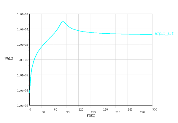
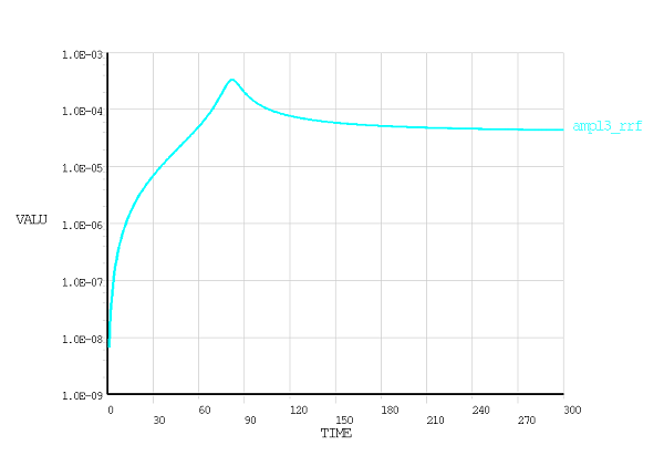
This example demonstrates the response of a Jeffcott rotor to mass unbalance excitation. It illustrates the equivalence between the static response in the rotating reference frame and the synchronous excitation (SYNCHRO command) in the stationary reference frame.
The model is the same as that shown in Example: Campbell Diagram Analysis of a Jeffcott Rotor, except damping is added in the bearings. This introduces rotating damping terms in the rotating reference frame analysis.
In this example, a force due to a fictive mass unbalance is acting on the mass. The response is calculated over a frequency range of 0 to 300 Hz. POST26 commands are used to output amplitude versus frequency/time graphs.
Inertia properties of the mass:
| Mass = 25 kg |
| Inertia (XX,YY) = 5 kg·m2 |
| Inertia (ZZ) = 10 kg·m2 |
Shaft length: 1 m
Bearing stiffness: 4e+6 N/m
Bearing damping: 1e+3 N·s/m
Excitation force amplitude (mass unbalance multiplied by eccentricity): 1e-3 kg·m
/title, Unbalance Response of a Jeffcott Rotor

! ** parameters

mass = 25
iz = 10
ix = 5
iy = 5
k = 4e+6
c = 1e+3
pi = acos(-1)
nstep = 300
f0 = 1e-3

/prep7

n,1,0,0,0
n,2,0,0,1
n,3,0,0,0.2

et,1,mass21             ! fake mass for CERIG 6 dofs
r,1
type,1
real,1
e,1
e,2

et,2,mass21
r,2,mass,mass,mass,ix,iy,iz
type,2
real,2
e,3

cerig,3,all,all

n,100,,,0
n,110,,,1

et,3,combi214           ! bearing
r,3,k,k,,,c,c
type,3
real,3
e,100,1
e,110,2

d,all,uz,0
d,all,rotz,0
d,100,all,0
d,110,all,0

esel,,type,,2
cm,masscm,elem
allsel,all
finish
save

! *** SYNCHRO ANALYSIS IN SRF

/solu
antype,harmonic
hropt,full
harfr,0,300
nsubst,nstep
kbc,1
f,3,fx,f0
f,3,fy,,-f0
coriolis,on,,,on
synchro
omega,,,1.0
solve
finish

/post26
nsol,2,3,u,x,ux3
nsol,3,3,u,y,uy3
realvar,4,2,,,ux3r
realvar,5,3,,,uy3r
prod,6,4,4,,ux3_2
prod,7,5,5,,uy3_2
add,8,6,7,,ux3_2+uy3_2
sqrt,9,8,,,ampl3_srf
*get,max_srf_,VARI,9,EXTREM,VMAX
parsav
/show,png,rev
/gropt,logy,1
/xrange,0,300
plvar,9
finish

! *** STATIC ANALYSIS IN RRF

/clear, nostart
resume,,db
parres

dfrq = 1

/solu
antype,static
kbc,1
coriolis,on,,,,on
frq = dfrq
*do,iloop,1,nstep
/gopr
   time,frq
   omg = 2*pi*frq
   cmomega,masscm,,,omg
   ftot = f0*omg**2
   f,3,fx,ftot
   solve
   frq = frq + dfrq
*enddo
finish

/post26
nsol,2,3,u,x,ux3
nsol,3,3,u,y,uy3
prod,6,2,2,,ux3_2
prod,7,3,3,,uy3_2
add,8,6,7,,ux3_2+uy3_2
sqrt,9,8,,,ampl3_rrf
*get,max_rrf_,VARI,9,EXTREM,VMAX
/show,png,rev
/gropt,logy,1
/xrange,0,300
plvar,9
finish

! *** COMPARE MAXIMUM AMPLITUDE
*status,PRM_