


The following table shows all available loads for an acoustic analysis:
Table 8.3: Acoustic Loads
| Loads | FE Model Entities |
|---|---|
| Transfer admittance matrix | Nodes |
| Impedance sheet | Nodes |
| Equivalent surface source | Nodes |
| Temperature | Nodes or elements |
| Static pressure | Nodes |
| Surface port | Nodes |
| Mean flow velocity (not valid for 2D acoustic elements) | Nodes |
| Ambient Temperature | Nodes |
| Quiescent pressure | Nodes |
The loads can be applied on FE model entities.
Use of temperature and static pressure body load are discussed in Non-Uniform Ideal Gas Material.
The following related topics are available:
To avoid meshing a complicated perforated structure, introduce a 2 x 2 transfer admittance matrix to trim the complex perforated structures. Define the element material and name it as the trim element (TB,PERF,,,,YMAT). Transfer admittance matrices are available only in harmonic acoustic analyses.
The coupled trim element connects with both the structural element and uncoupled acoustic element. The uncoupled trim element connects with the uncoupled acoustic elements, as shown in the following figure:
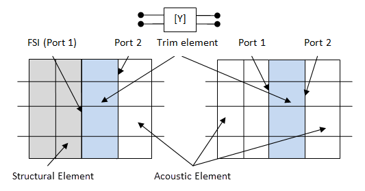
If the trim elements connect only to the uncoupled acoustic element, define the
port numbers of the 2 x 2 transfer admittance matrix with positive integers on a
pair of the opposite faces of the element
(SF,Nlist,PORT). The smaller port
number corresponds to port 1 of the 2 x 2 transfer admittance matrix and the greater
port number corresponds to port 2.
If one face of the coupled trim element is defined as the FSI interface
(SF,Nlist,FSI), it is assigned to
port 1 of the transfer admittance matrix, while its opposite face connecting with
the acoustic element should be defined by a port number
(SF,Nlist,PORT), corresponding to
port 2 of the transfer admittance matrix.
The following table shows the available transfer admittance matrix models:
Table 8.4: Transfer Admittance Matrix Models of Perforated Structures:
TB,PERF,,,,TBOPT
TBOPT
| Model | Input Parameters |
|---|---|---|
| YMAT | General transfer admittance matrix | 2 x 2 complex admittance matrix: Y11,Y12,Y21,Y22 |
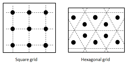
| HGYM | Hexagonal grid plate | Radius of hole, grid period, thickness, density, dynamic viscosity, ratio of inner and outer radius for cylindrical structure |
| SGYM | Square grid plate | Radius of hole, grid period, thickness, density, dynamic viscosity, ratio of inner and outer radius for cylindrical structure |
The following figure illustrates perforated plates with hexagonal and square grids:
The trim element is available only for hexahedral and prism elements.
In a hexahedral element, only a pair of opposite element faces can be defined as the ports. In a prism element, only two triangular element faces are used for the ports.
A pair of ports of the 2 x 2 transfer admittance matrix must be defined in the same element. No limitation exists on the trim element mesh size between two ports.
The 2 x 2 transfer admittance matrix can be symmetric or asymmetric. The program selects the correct solver for the specific transfer admittance matrix.
For a multi-layer perforated structure, if the individual transfer admittance matrix of each layer is known, convert the transfer admittance matrices to ABCD matrices. Multiply all ABCD matrices together. Convert the final ABCD matrix into the 2 x 2 transfer admittance matrix for the input.
Specify a frequency-dependent trim element with the general transfer admittance matrix as follows:
Two specified perforated structures with holes are present on the plate.
Specify a perforated structure with a square (TBOPT =
SGYM) or hexagonal (TBOPT = HGYM) grid as follows:
The program calculates the transfer admittance matrix during the solution in terms of the input parameters.
Example 8.23: Defining Uncoupled Trim Elements
tb,perf,2,,,YMAT                        ! define transfer admittance matrix
tbdata,1,y11r,y11i,y12r,y12i,y21r,y21i  ! complex 2 by 2 matrix
tbdata,7,y22r,y22i
tblist,perf,2                           ! list admittance matrix
…
esel,s,mat,,2                           ! element with YMAT
nsle,s                                  ! nodes in YMAT elements
nsel,s,loc,z,z1                         ! select nodes at z = z1
sf,all,port,1                           ! port 1
nsel,s,loc,z,z2                         ! select nodes at z = z2
sf,all,port,2                           ! port 2
…
nsel,s,loc,z,z3                         ! select nodes at z = z3 and 0
nsel,a,loc,z,0
sf,all,impd,z0                          ! impedance boundary
nsel,s,loc,z,0                          ! nodes at z = 0
sf,all,shld,-vn,                        ! normal velocity
Example 8.24: Defining Coupled Trim Elements with FSI
et,1,186                                ! structural element
et,2,220,,0                             ! coupled acoustic element
…
tb,perf,2,,,YMAT                        ! define transfer admittance matrix
tbdata,1,y11r,y11i,y12r,y12i,y21r,y21i  ! complex 2 by 2 matrix
tbdata,7,y22r,y22i
tblist,perf,2                           ! list admittance matrix
…
esel,s,mat,,2                           ! element with YMAT
nsle,s                                  ! nodes in YMAT elements
nsel,s,loc,z,z1                         ! select nodes at z = z1
sf,all,port,2                           ! port 2
nsel,s,loc,z,z2                         ! select nodes at z = z2
sf,all,fsi                              ! fsi interface (port 1)
Example 8.25: Defining Perforated Plates
et,1,220,,1                              ! uncoupled acoustic element
tb,perf,2,,,SGYM                         ! define square grid plate
tbdata,1,rad,period,thick,rho,visc,ratio ! input parameters
…
type,1                                   ! uncoupled fluid220
mat,2                                    ! perforated structure material
vmesh,all                                ! mesh volume
For more information, see Transfer Admittance Matrix in the Mechanical APDL Theory Reference.
The impedance sheet is a specification of the 2 x 2 transfer admittance matrix with continuous pressure and discontinuous normal velocity across the impedance sheet (for example, Y11=0.5Y, Y22=-0.5Y, Y12=Y21).
If your simulation has nearly continuous pressure and the full 2 x 2 transfer admittance matrix is unknown, see Impedance Sheet Approximation in the Mechanical APDL Theory Reference for a calculation of sheet impedance.
No element shape limitation exists on the impedance sheet.
Apply the impedance sheet to the interior surface of the model.
Define an impedance sheet via one of the following commands:
Example 8.26: Defining the Impedance Sheet
nsel,s,loc,z,0     ! nodes at z = 0
bf,all,impd,rs,xs  ! complex impedance sheet
The near and far fields beyond the FEA domain are of importance in acoustic analysis. Many design parameters (for example, the sound pressure level, radiated sound power, directivity or target strength) are based on the far-field values. The sound pressure field beyond the FEA domain can be calculated using the surface equivalence principle: the sound pressure field exterior to a given surface can be exactly represented by an equivalent source placed on that surface and allowed to radiate into the region external to that surface.
The equivalent source surface is available only for the near- and far-field parameters in a harmonic analysis.
For problems requiring near- and far-field computations, first define an equivalent source surface in the preprocessor. The surface must enclose the radiator or scatter, except for symmetry planes. Equivalent sources are calculated and stored on the surface, enabling quick calculation of near- and far-field information in the postprocessor.
For radiation and scattering problems, use an absorbing boundary condition (ABC).
For radiation problems, use perfectly matched layers (PML) or irregular perfectly matched layers (IPML), absorbing elements (FLUID130), or the far-field radiation boundary (INF).
For scattering problems, use either PML/IPML or the far-field radiation boundary (INF).
The equivalent source surface may be between the radiator or scatter and the PML or IPML region. Define an equivalent source surface using a surface boundary load with the flag MXWF. When applying a MXWF surface load, be sure to define an equivalent source surface. If no equivalent source surfaces are defined, the program flags the PML or IPML interface, absorbing element surface, or radiation boundary as the equivalent source surface. Do not flag any surface on a symmetry plane (for example, the Y-Z and X-Z planes in Figure 7.3: PML Enclosure).
Flag an equivalent source surface as follows:
Following is an alternate method for flagging an equivalent source surface:
Do not apply the surface flag via the SFA command, which transfers the surface flag to adjacent elements on either side of the equivalent source surface and can lead to erroneous results.
For more information, see Acoustic Output Quantities in the Mechanical APDL Theory Reference
If the APORT command is used to launch or terminate a specified mode in the acoustic duct, you can apply an exterior surface port on the exterior surface of the model and an interior surface port on the interior surface of the model.
Define an exterior surface port via the following command:
SF,
Nlist,PORT,PortNum
Define an interior surface port via the following command:
BF,
Node,PORT,PortNum
To indicate the ports of a transfer admittance matrix, issue the
SF,Nlist,PORT command
only. If the sound power is required after the solution, apply
the port number to the inlet and outlet before the solution.
To also define the impedance, issue the
SF,Nlist,IMPD command.
Example 8.27: Defining a Surface Port
nsel,s,loc,z,0                  ! nodes at z = 0
sf,all,port,1                   ! port 1 (exterior port)
aport,1,rect,11,1.,0,0,d,d,1,0  ! source port with rectangular (0,0) mode
nsel,s,loc,z,1                  ! nodes at z = 1
bf,all,port,2                   ! port 2 (interior port)
aport,2,rect,11,0,0,0,d,d,1,0   ! output port with rectangular (0,0) mode
When the acoustic fluid is not at rest, the mean flow will affect the propagation of the acoustic wave in the medium. To activate the solver taking the mean flow effect into account, the mean flow velocity must be defined on the model nodes. If the mean flow velocity is known, issue the following command:
BF,
Nlist,VMEN,v0x,v0y,v0z
Example 8.28: Defining Mean Flow
nsel,all                   ! Select all nodes
bf,all,vmen,1.0,0.0,0.0    ! Set mean flow v = (1,0,0)
Tabular input can be used to define the mean flow velocity. See the BF command for details. The mean flow velocity can be defined in the element coordinate system (ESYS).
Note: The mean flow effect is invalid for 2D acoustic elements.
For more information, see Solving the Convective Wave Equation for the Mean Flow Effect.
To define nodal ambient temperature for the non-uniform ideal gas material and the viscous-thermal full linear Navier-Stokes equations (FLNS) model, issue the following BF command:
BF,Nlist,TEMP,t0
Example 8.29: Defining Ambient Temperature
nsel,all              ! Select all nodes
bf,all,temp,20        ! Set temperature to 20 °C
toffst,273            ! Offset from absolute zero to zero
In the viscous-thermal FLNS model, the BF,,TEMP command defines quiescent temperature.
The TOFFST command specifies the temperature offset from absolute zero to zero.
Tabular input can be used to define the temperature. See the BF command for details.
The quiescent pressure refers to the environment pressure in the static state. The standard atmospheric pressure is 1.01325 x 10⁵ Pa. To define nodal quiescent pressure for the Non-Uniform Ideal Gas Material and the viscous-thermal Full Linear Navier-Stokes Equations (FLNS) Model, issue the following BF command:
BF,Nlist,SPRE,p0
Example 8.30: Defining Quiescent Pressure
nsel,all              ! Select all nodes
bf,all,spre,101325    ! Set quiescent pressure