


Sound excitation sources are fundamental to an acoustic analysis. You can introduce sound excitation sources via:
Specified pressure or energy (for a diffusion equation solution) at nodes (D)
Normal velocity (in a harmonic analysis or in a transient analysis solved with the velocity potential formulation) or acceleration (in a transient analysis solved with the pressure formulation) on the exterior surface of the domain (SF)
Arbitrary velocity (in a harmonic analysis or in a transient analysis solved with the velocity potential formulation) or acceleration (in a transient analysis solved with the pressure formulation) on the exterior surface of the domain (BF)
Analytic incident wave sources (AWAVE)
Mass source (harmonic analysis), mass source rate (transient analysis), or power source (diffusion equation solution) at nodes, along lines, on surfaces, or in volumes (BF)
Incident diffuse sound field (DFSWAVE)
Force potential with mean flow effect (BF)
The following table shows all excitation sources available for acoustic analysis:
Table 8.1: Acoustic Excitation Sources
| Excitation Sources | FE Model Entities |
|---|---|
| Pressure or energy density | Nodes |
| Outward normal velocity (acceleration) | Nodes |
| Arbitrary nodal velocity (acceleration) | Nodes or elements |
| Analytic incident wave sources | Not applicable |
| Mass sources or power source | Nodes |
| Diffuse sound field (not valid for 2D acoustic elements) | Not applicable |
| Acoustic duct port | Nodes |
| Force potential (not valid for 2D acoustic elements) | Nodes |
| Velocities in viscous-thermal acoustics | Nodes |
| Temperature in viscous-thermal acoustics | Nodes |
| Pressure in viscous-thermal acoustics | Nodes |
| Shear viscous force in viscous-thermal acoustics and poroelastic acoustics | Nodes |
| Volumetric body force in viscous-thermal acoustics | Nodes |
| Heat flux in viscous-thermal acoustics | Nodes |
| Volumetric heat source in viscous-thermal acoustics | Nodes |
| Displacements in poroelastic acoustics | Nodes |
Excitation sources can be applied on the finite element model entities.
The following detailed descriptions of the available excitations are available:
- 8.1.1. Pressure or Energy Density Excitation
- 8.1.2. Outward Normal Velocity (Acceleration) Excitation
- 8.1.3. Arbitrary Velocity (Acceleration) Excitation
- 8.1.4. Analytic Incident Wave Sources
- 8.1.5. Mass Source, Mass Source Rate, or Power Source
- 8.1.6. Random Excitation with Diffuse Sound Field
- 8.1.7. Specified Mode Excitation in an Acoustic Duct
- 8.1.8. Force Potential for Mean Flow Effect
- 8.1.9. Excitation Sources in Viscous-Thermal Acoustics
- 8.1.10. Excitation Sources in Poroelastic Acoustics
For general information about applying loads, see Loading in the Basic Analysis Guide.
Pressure excitation (D,Node,PRES)
behaves as a Dirichlet pressure boundary (Pressure Boundary).
When applying pressure excitation, the pressure is enforced to a given value. Sound pressure reflected by other objects back to the excitation point cannot be taken into account.
Pressure excitation can be used only under conditions where the effect of reflected sound pressure is not required.
In a diffusion equation solution, the acoustic energy density
can be constrained (D,Node,ENKE) as a
Dirichlet boundary condition. The initial condition is defined by the command
IC,Nlist,ENKE).
Outward normal velocity or acceleration can be applied to
the exterior surface of the model
(SF,Nlist,SHLD). The velocity
excitation is valid in a harmonic analysis or in a transient analysis solved with
the velocity potential formulation. The acceleration excitation is valid in a
transient analysis solved with the pressure formulation.
To use normal velocity excitation in a transient analysis, you must set KEYOPT(1) = 4 on the acoustic element to activate the velocity potential formulation for the solution.
Apply a minus sign to the outward normal velocity if an inward normal velocity is required.
For a harmonic analysis, a complex normal velocity to the surface is defined by the amplitude and phase angle. The program solves for the pressure on the normal velocity excitation surface.
Normal velocity excitation exists either on the structural surface or on the
transparent pressure wave port on which the incident wave propagates into the
acoustic domain and the reflected wave backs to the infinity. To absorb the
reflected wave on the transparent port, apply the impedance boundary to the port
surface (SF,Nlist,IMPD or
SF,Nlist,INF) along with the
velocity excitation. To distinguish the transparent wave port from the structural
surface, specify the transparent port surface
(SF,Nlist,PORT).
The following command applies outward normal velocity or acceleration to the nodes of the FE model:
SF,
Nlist,SHLD,Value,Value2
Example 8.1: Defining the Normal Velocity and Impedance BC on a Transparent Wave Port
nsel,s,loc,z,0        ! select nodes at z = 0
sf,all,shld,vn,ang    ! complex normal velocity
sf,all,impd,z0        ! impedance boundary
sf,all,port,1         ! transparent port
Example 8.2: Defining the Normal Velocity and Impedance BC on a Structural Surface
nsel,s,loc,z,0       ! select nodes at z = 0
sf,all,shld,vn,ang   ! complex normal velocity
sf,all,impd,z0       ! impedance boundary
Example 8.3: Defining the Frequency Dependency of the Normal Velocity of Acceleration
Use tables (*DIM) in the SF command to define the frequency dependency of the normal velocity of acceleration, as shown:
*dim,vn,TABLE,2,1,1,FREQ       ! normal velocity table
*dim,ang,TABLE,2,1,1,FREQ      ! angle table
vn(1,0,1)=FreqB                ! beginning frequency
vn(2,0,1)=FreqE                ! ending frequency
vn(1,1,1)=vn1                  ! normal velocity at FreqB
vn(2,1,1)=vn2                  ! normal velocity at FreqE
ang(1,1,1)=ang1                ! phase angle at FreqB
ang(2,1,1)=ang2                ! phase angle at FreqE
nsel,s,loc,z,0                 ! select nodes at z = 0
sf,all,shld,%vn%,%ang%         ! tabular complex vn
An arbitrary velocity or acceleration can be applied to the
nodes on the exterior surface of the model
(BF,Node,VELO). The velocity
excitation is valid in a harmonic analysis or in a transient analysis solved with
the velocity potential formulation. The acceleration excitation is valid in a
transient analysis solved with the pressure formulation.
To use arbitrary velocity excitation in a transient analysis, you must set KEYOPT(1) = 4 on the acoustic element to activate the velocity potential formulation for the solution.
The arbitrary velocities are projected to the outward normal direction on the excitation surface after interpolation during an acoustic solution. For a harmonic analysis, a complex velocity is defined by the amplitudes and phase angles of the components.
The arbitrary velocity or acceleration can be defined in a local Cartesian coordinate system (LOCAL), then assigned to the elements (VATT or ESYS prior to meshing or EMODIF after meshing). The program solves for pressure on the velocity excitation surface. If the reflected sound pressure waves that are passing through the velocity excitation surface are simulated, apply the impedance boundary condition to the excitation surface. The arbitrary velocity excitation exists either on the structural surface or on the transparent pressure wave port.
The following command applies arbitrary velocity to the nodes of the FE model:
BF,
Node,VELO,Vx,Vy,Vz,AngX,AngY,AngZ
Example 8.4: Defining the Arbitrary Velocity and Impedance BC on a Transparent Wave Port
et,1,220,,1                          ! uncoupled acoustic element
local,11                             ! local coordinate
esys,11                              ! use local as element esys
…
nsel,s,loc,z,0                       ! select nodes at z = 0
bf,all,velo,vx,vy,vz,angx,angy,angz  ! complex arbitrary velocity
sf,all,impd,z01                      ! impedance boundary
sf,all,port,1                        ! transparent port
Example 8.5: Defining the Frequency Dependency of the Arbitrary Velocity or Acceleration
Use tables (*DIM) in the BF command to define the frequency dependency of the arbitrary velocity or acceleration, as shown:
*dim,vx,TABLE,2,1,1,FREQ                  ! vx table
*dim,vy,TABLE,2,1,1,FREQ                  ! vy table
*dim,vz,TABLE,2,1,1,FREQ                  ! vz table
*dim,ax,TABLE,2,1,1,FREQ                  ! angle x table
*dim,ay,TABLE,2,1,1,FREQ                  ! angle y table
*dim,az,TABLE,2,1,1,FREQ                  ! angle z table
vx(1,0,1)=FreqB                           ! beginning frequency
vx(2,0,1)=FreqE                           ! ending frequency
vx(1,1,1)=vx1                             ! vx at FreqB
vx(2,1,1)=vx2                             ! vx at FreqE
vy(1,1,1)=vy1                             ! vy at FreqB
vy(2,1,1)=vy2                             ! vy at FreqE
vz(1,1,1)=vz1                             ! vz at FreqB
vz(2,1,1)=vy2                             ! vz at FreqE
ax(1,1,1)=vx1                             ! angle x at FreqB
ax(2,1,1)=vx2                             ! angle x at FreqE
ay(1,1,1)=vy1                             ! angle y at FreqB
ay(2,1,1)=vy2                             ! angle y at FreqE
az(1,1,1)=vz1                             ! angle z at FreqB
az(2,1,1)=vy2                             ! angle z at FreqE
nsel,s,loc,z,0                            ! select nodes at z = 0
bf,all,velo,%vx%,%vy%,%vz%,%ax%,%ay%,%az% ! complex velocity table
Acoustic analyses often use wave sources with analytic functions in harmonic analysis. The following table shows all available analytic wave sources for acoustic analyses:
Table 8.2: Acoustic Analytic Incident Wave Sources
| Wave Sources | Comments |
|---|---|
| Planar wave | Plane wave with the incident φ and θ in the global spherical coordinate system from infinity |
| Monopole or pulsating sphere | Spherical wave from the origin (xs,ys,zs) |
| Dipole | Consists of two monopoles or pulsating spheres with opposite signs and a small separation |
| Back enclosed loudspeaker | Loudspeaker with back enclosure acting as a monopole |
| Bare loudspeaker | Loudspeaker without back enclosure acting as a dipole |
To define various incident wave sources, issue the AWAVE command
Specify the integer number (WaveNum) or an acoustic
incident wave inside or outside of the model. Valid values are 1 through 20. One or
more wave types can be selected. The amplitude of the pressure or normal velocity is
used for the excitation.
A planar wave can be defined in terms of the amplitude and the spatial incident angles in the global spherical coordinate system, as shown in this figure:
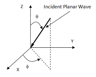
Because the incident planar wave is approximated by the far-field wave front of a source far from the receiver, both the initial phase angle and the source original are ignored.
Specify the analytic incident wave sources and select either the total pressure field or the scattered field solver in an acoustic scattering analysis.
If the scattered parameter is required and the scattered pressure field is much smaller than the incident pressure field, use the scattered pressure field solver (ASOL,SCAT) to avoid numerical errors. Control the output result as needed for either the total or scattered nodal pressure in the model (ASCRES).
Specify incident wave sources as external sources (Opt2
= EXT on the AWAVE command) if a
scattering analysis is needed.
When analytic incident wave sources are used inside the model
(Opt2 = INT on the
AWAVE command), only the scattered pressure field solver is
activated, regardless of whether the ASOL,SCAT command is issued.
The source origin must be located inside the model. The plane wave incident source cannot be used inside the model.
The uniform normal velocity on the cross section can be used to launch the plane wave. When analytic incident wave sources are located inside the model, the nodal total pressure is always output, even though the scattered field solver is used.
Example 8.6: Defining an Internal Pulsating Sphere with Normal Velocity
block,0,xs,0,ys,0,zs                        ! geometry of model
…
awave,1,mono,velo,int,v0,ang,xs/2,ys/2,zs/2 ! incident wave inside of model
Example 8.7: Defining an External Dipole with Pressure
block,0,xs,0,ys,0,zs                       ! geometry of model
…
awave,1,dipole,pres,ext,p0,ang,-xs,-ys,-zs ! incident wave outside of model
It is not necessary to assign the internal analytic incident wave sources to the FE nodes. It is convenient to use the internal analytic incident wave sources rather than meshing the wave source structure, such as a pulsating sphere.
For more information, see Pure Scattered Pressure Formulation in the Mechanical APDL Theory Reference.
To excite sound waves in an acoustic model, use a mass source (harmonic analysis or a transient analysis solved with the velocity potential formulation), a mass source rate (transient analysis solved with the pressure formulation), or a power source (diffusion equation solution).
The mass source is input by defining up to one scalar quantity
(Lab = MASS on the BF command) and
a phase angle. The mass source is specified at nodes (BF).
For a volume mass source (kg/(m3*s)), specify the mass source on the volumetric nodes.
For a surface mass source (kg/(m2*s)), specify the mass source on at least three nodes on an element face. The surface mass source must coincide with the element's faces.
For a line mass source (kg/(m*s)), specify the mass source at two nodes connected by an element edge. The line mass source must coincide with the element's edges.
A point mass source (kg/s) must be at the element's nodes.
To use mass source excitation in a transient analysis, you must set KEYOPT(1) = 4 on the acoustic element to activate the velocity potential formulation for the solution.
In general, a mass source launches the pressure wave in all directions. For a propagating or resonant system, a mass source can be used to excite the propagating modes or resonant modes of the structure.
Only proper modes can exist in the structure. To reduce the parasitic modes, choose the distribution of the mass source based on the pressure distribution of the excited mode.
When a mass source is applied to an exterior surface, the excited pressure is determined by p = qsc0. On an exterior or interior transparent port, the excited pressure is given by p = qsc0 / 2.
Example 8.8: Defining a Surface Mass Source
nsel,s,loc,z,0               ! select nodes at z = 0
bf,all,mass,masmag,masang    ! complex mass source
Example 8.9: Defining the Frequency Dependency of the Arbitrary Mass Source or Mass Source Rate
Use tables (*DIM) in the BF command to define the frequency dependency of the arbitrary mass source or mass source rate, as shown:
*dim,masmag,TABLE,2,1,1,FREQ      ! mass source amplitude table
*dim,masang,TABLE,2,1,1,FREQ      ! mass source angle table
masmag (1,0,1)=FreqB              ! beginning frequency
masmag (2,0,1)=FreqE              ! ending frequency
masmag (1,1,1)=vx1                ! amplitude at FreqB
masmag (2,1,1)=vx2                ! amplitude at FreqE
masang (1,1,1)=vz1                ! angle at FreqB
masang (2,1,1)=vy2                ! angle at FreqE
nsel,s,loc,z,0                    ! select nodes at z = 0
bf,all,mass,% masmag%,%masang%    ! complex mass source table
For more information, see Mass Source in the Wave Equation in the Theory Reference.
In a diffusion equation solution, the omnidirectional power source can be defined with the BF,,MASS command. The units for the volumetric, surface, line and point power sources are (W/m3), (W/m2), (W/m) and (W), respectively.
For more information, see Power Source in the Diffusion Equation in the Theory Reference.
The diffuse sound field is approached by the asymptotic model summing a high number of uncorrelated plane waves with random phases from all directions in free space. The DFSWAVE command defines the diffuse sound field.
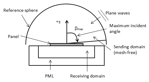
The incident space of the diffuse sound field is mesh-free. A reference sphere
related to the structural panel defines the incident plane waves. The radius R of
the reference sphere should be at least 50 times the maximum dimension of the
structural panel. The energy of the diffuse sound field uniformly distributes on the
reference sphere surface in all directions. The sphere surface is equally divided
into N elementary surfaces.
The plane center of the structural panel should be located at the origin of the local Cartesian coordinate system (LOCAL) (defaults to the global Cartesian coordinate system). The +z axis of the Cartesian coordinate system must be consistent with the panel’s outward normal unit vector on the panel’s incident diffuse sound field side. The structural panel is meshed by solid or shell elements.
The receiving domain is meshed by acoustic elements and truncated by artificially matched layers (PML or IPML) or by absorbing elements, as shown in this figure:
If the effect of the acoustic fluid on the structural panel can be ignored, it is not necessary to create a receiving acoustic domain. The radiated sound far-field is calculated in the postprocessor (PRFAR,PLAT or PLFAR,PLAT) once the structural panel model is solved with the flagged equivalent source surface (SF,,MXWF).
In practice, the sphere surface is divided into M parallel rings along the z axis of a local Cartesian coordinate system, and the program generates the elementary surfaces, each having nearly the same area.
When defining the diffuse sound field, the DFSWAVE command specifies the local coordinate system number, the radius of the reference sphere, the reference power spectral density, mass density of the incident space, the sound speed in the incident space, the maximum incident angle of the plane waves, the number of the parallel rings, and the sampling options.
To excite the vibro-acoustics system, generate the SURF154 surface element on the surface of the structural elements.
The symmetry of a panel structure cannot be used to reduce the simulation size, as the incident plane waves have varying random phase angles.
To initiate multiple solutions (load steps) for random acoustics analysis with
multiple samplings, issue the MSOLVE command. The process is
controlled by the norm convergence tolerance
(VAL1 on
MSOLVE) or the number of multiple solutions if the
number of solution steps reaches the number specified
(NUMSLV
on MSOLVE). The program checks the norm
convergence by comparing two averaged sets of radiated sound powers with the
interval of the norm (VAL2 on
MSOLVE) over the frequency range.
To calculate the average transmission loss for multiple sampling phases at each frequency over the frequency range, issue the PRAS or PLAS command.
Example 8.10: Diffuse Sound Field Analysis of a Panel
et,1,220,,0          ! coupled acoustic element
et,2,220,,1,,1       ! acoustic PML element
et,3,281             ! structure shell element
et,4,154             ! surface element
…
cm,nod1,node         ! group vibro-acoustics FSI interface nodes
sf,all,fsi           ! flag FSI interface
…
sectype,2,shell
secdata,0.005,2
cmsel,s,nod1         ! select FSI interface nodes
type,3
mat,2
secn,2
esurf                ! generate shell element
alls

esel,s,type,,3       ! select shell element
type,4
mat,2
esurf                ! generate surface element
…

! define diffuse sound field
dfswave,0,15,1,1.225,340,90,20,all
!
finish
/solu
antype,harmic
harfrq,100,200
nsubst,100
msolve,5             ! five samples
finish

/post1
pras,dfstl,avg       ! print transmission loss
plas,dfstl,avg       ! plot transmission loss
finish
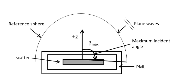
If the incident diffuse sound field projects onto the objects and is scattered, the scattering analysis can be performed without using the SURF154 surface element. The infinite scattering open domain is meshed by acoustic elements and truncated by artificially matched layers (PML or IPML), as shown in this figure:
The scattered pressure field solver (ASOL,SCAT) and the nodal scattered pressure solution (ASCRES) are invalid for the scattering analysis of the diffuse sound field.
Note: The solution for the diffuse sound field is not valid for 2D acoustic elements.
For more information, see Random Acoustics in the Mechanical APDL Theory Reference.
A single mode or multiple modes may exist in the acoustic duct. Launching a specified acoustic mode into a guided acoustic wave system with discontinuities excites multiple propagating or evanescent modes, depending on the working frequency and geometrical dimension of the duct.
If the lowest order mode is launched and the higher order modes decay as the parasitic evanescent modes near the discontinuities, the acoustic port can be used to terminate the inlet or outlet with the specified mode. While the multiple propagating modes are excited and propagate in the acoustic duct, PML or IPML should be used for the domain truncation.
Define the property of an analytic modal port via the following command:
APORT,
PortNum,Label,KCN,PRES,PHASE,--,VAL1,VAL2,VAL3,VAL4
The available analytic port types are planar wave, rectangular duct, circular duct, and coaxial duct.
Example 8.11: Defining Acoustic Ports in a Duct
et,1,220,,            ! acoustic element
et,2,220,,1,,1        ! acoustic PML element
et,3,186              ! structural element
...
nsel,s,loc,z,0
nsel,a,loc,z,1
sf,all,fsi            ! fsi interface

nsel,s,loc,x,-1
nsel,a,loc,x,1
nsel,r,loc,z,-5,5
cpcyc,all,,,2         ! coupled nodes for PBC
...
nsel,s,loc,z,4
bf,all,port,1                 ! flag interior port 1
aport,1,plan,0,p0,0,0,0,theta ! plane wave source port
nsel,s,loc,z,-4)
bf,all,port,2                 ! flag interior port 2
aport,2,plan,0,0,0,0,0,theta  ! plane wave output port

nsel,s,loc,z,-5
nsel,a,loc,z,5
d,all,pres,0                  ! zero pressure on PML exterior surface
Note that the transverse cross section of the acoustic port must be located on the x-y plane in the defined local coordinates system (LOCAL).
The low-order FLUID30 element does not support the higher modes in the coaxial duct.
For more information, see Analytic Port Modes in a Duct in the Mechanical APDL Theory Reference.
The complex force potential, defined by the BF,,UFOR command, is introduced to represent the body force in the convective wave equation when the mean flow effect is considered. The load vector due to the force potential is calculated in the element volume.
Example 8.12: Defining Potential Force in a Volume
nsel,s,loc,x,0,1     ! select nodes from x = 0 to 1
nsel,r,loc,y,0,1     ! reselect nodes from y = 0 to 1
nsel,r,loc,z,0,1     ! reselect nodes from z = 0 to 1
bf,all,ufor,ur,ui    ! complex force potential
Note: The force potential is not valid for 2D acoustic elements.
For more information, see Governing Equations with Mean Flow Effect in the Theory Reference.
There are several ways to apply the excitation sources in a viscous-thermal acoustic analysis, including constraints, and surface and volumetric sources. These are described in:
For more information on viscous-thermal acoustics, see The Full Linear Navier-Stokes (FLNS) Model in the Theory Reference.
The acoustic velocity excitation, defined by the command
D,Node,VX/VY/VZ, behaves as
the Dirichlet boundary condition.
When applying velocity excitation, the velocities are enforced to defined values during the solution. The NROTAT command can be used to define the normal or tangential velocity components on the surfaces.
Example 8.13: Defining Velocities on Nodes
nsel,s,loc,x,0,1     ! Select nodes from x = 0 to 1
d,all,vx,0           ! Zero x component of velocity
d,all,vy,0           ! Zero y component of velocity
d,all,vz,1,2         ! Complex z component of velocity
The temperature constraint, defined by the command
D,Node,TEMP, specifies the
temperature values on the nodes as the Dirichlet boundary condition.
Example 8.14: Defining Temperature on Nodes
nsel,s,loc,x,0,1     ! Select nodes from x = 0 to 1
d,all,temp,0         ! Zero temperature
As an acoustic source, the surface pressure that is approximately equal to the normal stress is exerted on the exterior surface of the FLNS model to excite the acoustic wave in the viscous-thermal media. Use the command SF,,PRESS to define this pressure.
Since the degree of freedom pressure is used as an auxiliary variable for avoiding the spurious solution, it is not necessary to constrain the pressure with the D,,PRES command in the FLNS model. Other boundary conditions, such as the impedance boundary, can be applied to the surface with the pressure load.
Example 8.15: Defining Pressure on a Surface
nsel,s,loc,x,0,1     ! Select nodes from x = 0 to 1
sf,all,pres,1        ! Pressure = 1
sf,all,impd,z0       ! Acoustic impedance boundary
The vectoral shear viscous force, defined by the command BF,,SFOR, can be applied on the exterior surface of the FLNS model as the excitation source.
The components of the shear force should be defined in the current element coordinates (ESYS). Other boundary conditions, such as the impedance boundary, can be applied to the surface with shear force load.
Example 8.16: Defining Shear Viscous Force on a Surface
esys,0               ! Global Cartesian coordinates
nsel,s,loc,x,0,1     ! Select nodes from x = 0 to 1
bf,all,sfor,0,1,1    ! Shear force
sf,all,impd,z0       ! Acoustic impedance boundary
Use the F command to define volumetric force density on nodes. Units should be in terms of force/length3. For more information, see The Full Linear Navier-Stokes (FLNS) Model in the Theory Reference.
Example 8.17: Defining Volumetric Force Density on Nodes
nsel,s,loc,x,0,1     ! Select nodes from x = 0 to 1
f,all,fx,1           ! x component of force density
The thermal surface heat flux acts as the thermal source. Use the command SF,,CONV to define the heat flux on the exterior surface of the FLNS model.
Other boundary conditions, such as the impedance boundary, can be applied to the surface with the heat flux load.
Example 8.18: Defining Heat Flux on a Surface
nsel,s,loc,x,0,1     ! Select nodes from x = 0 to 1
sf,all,conv,1        ! Heat flux
sf,all,impd,z0       ! Acoustic impedance boundary
Use the command BF,,HFLW to define the volumetric heat source on nodes.
Example 8.19: Defining Volumetric Heat Source on Nodes
nsel,s,loc,x,0,1     ! Select nodes from x = 0 to 1
bf,all,hflw,1        ! Volumetric heat source
There are several ways to apply the excitation sources in a poroelastic acoustic analysis, including constraints and surface sources. These are described in:
For more information on poroelastic acoustics, see Poroelastic Acoustics in the Theory Reference.
Imposing a pressure field implies the continuity of the total normal stress and the continuity of the pressure on the surface. Use the command D,,PRES. The imposed pressure is a simple way to simulate the normal incidence of plane wave from air.
Example 8.20: Defining Pressure on a Surface
nsel,s,loc,x,0,1     ! Select nodes from x = 0 to 1
d,all,pres,1         ! Pressure = 1
Imposing a displacement field implies the continuity between the solid phase displacement and the imposed displacement, and the continuity of the normal displacement between the solid phase and normal fluid. Use the command D,,UX (or UY or UZ). The imposed displacement is a simple way to simulate the motion of a piston.
Example 8.21: Defining an Imposed Displacement
nsel,s,loc,x,0,1     ! Select nodes from x = 0 to 1
d,all,ux,1           ! x-component displacement = 1
d,all,uy,1           ! y-component displacement = 0
d,all,uz,1           ! z-component displacement = 0
The vectoral shear force, defined by the command BF,,SFOR, can be applied on the exterior surface of the poroelastic model as the excitation source.
The components of the shear force should be defined in the current element coordinate system (ESYS). Other boundary conditions, such as the pervious porous boundary, can be applied to the surface with shear force load.
Example 8.22: Defining Shear Viscous Force on a Surface
esys,0               ! Global Cartesian coordinates
nsel,s,loc,x,0,1     ! Select nodes from x = 0 to 1
bf,all,sfor,0,1,1    ! Shear force
sf,all,perm,k0       ! Pervious porous boundary