


An absorbing boundary condition (ABC) absorbs the outgoing pressure wave so that there are no reflections back into the FEA computational domain. The artificially matched layers are the layers of pressure-wave-absorbing elements designed for the mesh truncation of an open FEA domain with a homogeneous isotropic material in a modal, harmonic, or transient analysis. Artificially matched layers are a transparent artificial anisotropic material which is heavily lossy to incoming pressure waves.
Using artificially matched layers can reduce the size of the computational domain significantly with very small numerical reflections. A region of the artificially matched layers is backed by a soft-sound boundary condition (p = 0, or the velocity potential Φ = 0 for the convective wave equation).
There are two methods for modeling artificially matched layers:
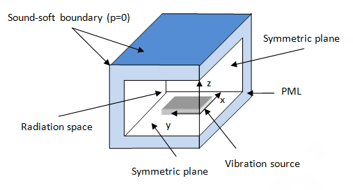
The perfectly matched layers (PML) are located inside a cubic enclosure. The PML materials are specified in face, edge, and corner regions in a three-dimensional model.
If the pressure wave should be absorbed in only one direction, such as in a traditional tube, construct a 1D PML region in the global Cartesian coordinate system or a local Cartesian coordinate system, as shown in this figure:

To define PML elements, issue the ET command to specify the desired fluid element type (FLUID30, FLUID220, FLUID221, FLUID243, or FLUID244). For that element type, also set the appropriate KEYOPT(4) value prior to meshing the PML region:
| KEYOPT(4) = 1 in a harmonic or modal solution |
| KEYOPT(4) = 3 in a transient solution |
Use any element shape to mesh the PML block.
More than one 1D PML regions can exist in a model. The PML element coordinate system (PSYS) uniquely identifies each PML region. Define a Cartesian coordinate system (LOCAL) with one axis in the wave-propagating direction, then assign the coordinate system to the elements in the PML region (VATT or PSYS prior to meshing, or EMODIF after meshing).
Example 7.10: Defining PML Elements in a Local Coordinate System
et,11,200,6                   ! Mesh element
et,1,30,,1                    ! Normal fluid30
et,2,30,,1,,1                 ! PML fluid30
…
local,11,0,2,3,4,50,-60,135   ! Local coordinate
wpcsys,,11
rect,0,l,-d/2,d/2             ! Area in local cs
rect,l,l+dpml,-d/2,d/2        ! Area in local cs
aglue,all
esize,h
type,11
amesh,all                     ! Mesh area with mesh200
asel,all
asel,u,,,3
esla
type,1                        ! Normal element
mat,1
esize,,2
vext,all,,,0,0,d,             ! 3d mesh with normal element
psys,11                       ! Activate local PML element coordinate
asel,s,,,3
type,2,                       ! PML element
mat,1
esize,,2
vext,all,,,0,0,d,             ! 3d mesh with PML element in psys 11
…
nsel,s,loc,x,l+dpml           ! Nodes backed to PML
d,all,pres,0.                 ! Zero pressure on boundary
A 3D PML region consists of layers of elements extending from the interior volume towards the open domain, as shown in this figure:
Construct a block about the origin in the global Cartesian coordinate system or a local Cartesian coordinate system. Align the edges of the 3D PML region with the axes of the Cartesian coordinate system.
To optimize the absorbing efficiency of the PML, construct the PML regions and apply the following parameters carefully:
Thickness of the PML region
Number of PML elements (≥ 3)
Attenuation parameters
Number of buffer elements between the PML region and objects or discontinuities. The buffer elements represent the propagating space of the sound wave.
More than two (≥ 2) buffer elements are recommended in harmonic or transient analysis. To avoid spurious modes, use one buffer element in modal analysis.
The attenuation from the PML interface to the PML exterior surface is a parabolic distribution that minimizes numerical reflections from the PML elements, as shown in this figure:
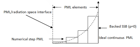
The numerical reflection is caused by the discretization of a continuous distribution of material from element to element. To obtain satisfactory numerical accuracy, use at least two layers of PML elements. The PML thickness may need to be greater than 1/10 of a wavelength.
Because a PML region acts as an infinite open domain, any boundary conditions and material properties must be carried over to the PML region. Material properties such as mass density and sound speed in the PML region must be identical to those of the adjacent interior region.
A sound-soft Dirichlet boundary with p = 0 or Φ = 0 must back all exterior surfaces of the PML region, except for symmetric surfaces with a rigid wall boundary condition. To specify a sound-soft boundary condition on the outer surfaces of the PML region, use the D,,PRES,0 command for a finite element model (the velocity potential Φ is assigned to the pressure degree-of-freedom label for the convective wave equation). The sound-soft or sound-hard boundary conditions can be applied on symmetric surfaces of a PML region.
The buffer elements between the PML region and a discontinuity or object in the domain are shown in the figure below.
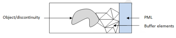
The PML can then absorb the outgoing wave effectively and minimize numerical reflections.
Because PML is an artificial anisotropic material, excitation sources are prohibited in the PML region.
The attenuation of the pressure wave in a PML region can be controlled. If desired, use the PMLOPT command to specify the normal reflection coefficient (harmonic) for propagating waves:
PMLOPT, PSYS,
Lab, Xminus,
Xplus, Yminus,
Yplus, Zminus,
Zplus, WOptXm,
WOptXp, WOptYm,
WOptYp, WOptZm,
WOptZp
The direction designations are Xminus,
Yminus, Zminus,
Xplus, Yplus, and
Zplus. The minus and plus refer to the negative and
positive directions along the Cartesian coordinate axes, respectively.
The WOptXm to
WOptZp arguments define the type of attenuated sound
wave and the associated PML parameter (s = α(x) – jβ(x)) in each
direction. Four scenarios are possible:
If only the propagating sound wave exists in a direction, the PML parameter is chosen in terms of the normal reflection coefficients (defaults to 1.E-3) with α=1.
If the evanescent sound wave decays in a direction, the PML parameter is set to s = α with α > 1 (defaults to 30).
The PML may absorb both the propagating and evanescent sound wave simultaneously with the program-defined coefficient α value.
The frequency-independent PML parameter is defined with the maximum lossy factor (defaults to 40), which is necessary for a modal solution.
If the propagating wave is absorbed in only one direction, define a 1D PML region
(Lab = ONE). In this case,
only the Xminus argument is necessary.
For a 3D PML region, a different normal reflection coefficient can be defined for
each direction (Xminus,
Yminus, Zminus,
Xplus, Yplus,
Zplus). Normal reflection coefficients default to
10-3 (-60 dB) for a harmonic or transient analysis. Normal reflection
coefficients should be less than 1.0. If only a very few PML layers are used (for
example, two or three), specifying a very small normal reflection coefficient (such
as -100 dB) may lead to significant numerical reflection.
Example 7.11: Defining 3D PML Parameters
The following example input defines 3D PML parameters as illustrated in Figure 7.3: PML Enclosure:
pmlxm=0                   ! No PML in –x direction
pmlxp=-40                 ! -40 dB in +x direction
pmlym=0                   ! No PML in –y direction
pmlyp=-40                 ! -40 dB in +y direction
pmlzm=-60                 ! -60 dB in –z direction
pmlzp=-60                 ! -60 dB in +z direction

! Define 3-d PML
pmlopt,0,three,pmlxm,pmlym,pmlzm,pmlxp,pmlyp,pmlzp
Repeat the PMLOPT command for additional PML regions. The PML may have a different number of elements in each direction.
The number of PML layers determines the absorbing efficiency of the PML region. An excessive number of PML elements significantly increases computational requirements. The number of PML layers (n) for acceptable numerical accuracy is determined by the following command:
PMLSIZE,
FREQB,FREQE,DMIN,DMAX,THICK,ANGLE
The following figure shows the relationship between
DMIN, DMAX, and
THICK:
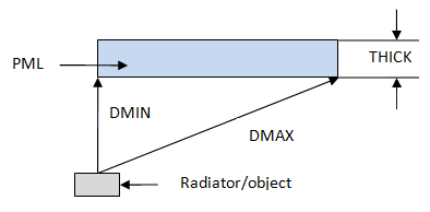
If n < 2, the number of layers is set to 2 to reduce numerical reflection. If n > 20, the number of layers is set to 20 to avoid an excessive number of PML elements.
Before meshing the model, issue the PMLSIZE command. If the thickness of the PML region is known, the command specifies an element edge length. If the thickness of the PML region is unknown, it specifies the number of layers (n). For further information, see the PMLOPT and PMLSIZE commands in the Command Reference.
PML may be necessary in cases where:
The impedance is unknown on exterior surfaces of the model, such as complex scatters.
Multiple propagating modes on the outlet surface are excited by discontinuities in the structure so that the defined impedance may not absorb all outgoing propagating modes.
Using the spherical second-order ABC leads to numerous elements or lesser accuracy.
High absorbing rate is required for greater numerical accuracy.
In most acoustic radiation and scattering applications, the open domain is fully enclosed by 3D PML, as shown in Figure 7.3: PML Enclosure. If the radiated acoustic field has no significant effect on the excitation source entity, however, the 3D PML can be used to locally enclose the open space near the radiation outlet, as shown in this figure:
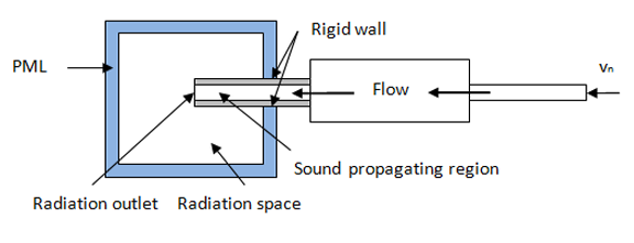
It is necessary to separate the PML region and sound-propagating region with the rigid wall, as the PML connects only to the infinity.
In a transient analysis, the additional auxiliary variables (degree-of-freedom labels VX, VY, VZ, and ENKE) are introduced on the nodes of PML elements. The program applies constraints for these additional variables on the PML elements.
For more information, see Perfectly Matched Layers (PML) in the Mechanical APDL Theory Reference.
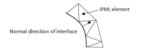
The locally conformed, irregular perfectly matched layers (IPML) are located inside a convex enclosure. The IPML material is specified based on the local normal direction of the IPML interface, as shown in the figure below.
IPML can be included in a modal, harmonic, or transient acoustic analysis. The use of the IPML is the same as discussed for PML (see Perfectly Matched Layers (PML)). Fewer buffering and absorbing elements are generated for IPML compared to PML. However, IPML may have worse absorption than PML. IPML does not support the pure scattered pressure formulation in radiation and scattering analyses.
To define IPML elements, issue the ET command to specify the desired fluid element type (FLUID30, FLUID220, FLUID221, FLUID243, or FLUID244). Set KEYOPT(4) = 2 or 4 for that element type prior to meshing the IPML region. Use any element shape to mesh the IPML region.
The IPML region is not related to any user-specified global or local coordinate system.
The construction of a 1D IPML region is similar to 1D PML construction (see Figure 7.2: 1D Multiple PMLs for Pipes).
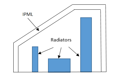
A 3D IPML region consists of elements extending from the interior convex-shaped volume towards the open domain, as shown in the figure below.
It is necessary to construct IPML as a convex region. To optimize the absorbing efficiency of the IPML, construct the IPML regions and apply the following parameters carefully:
Uniform thickness of the IPML region
Number of IPML elements (≥3)
Program-controlled attenuation parameters
Number of buffer elements between the IPML region and objects or discontinuities (≥2 for a harmonic or transient solution; = 1 for a modal solution)
The attenuation from the IPML interface to the IPML exterior surface is a parabolic distribution (see Figure 7.4: Attenuation Distribution).
Boundary conditions and material properties must be carried over into the IPML region. Material properties of the IPML must be identical to those of the adjacent interior region. Excitation sources are prohibited in the IPML region.
A sound-soft Dirichlet boundary with p = 0 or Φ = 0 must back all exterior surfaces of the IPML region, except for symmetric surfaces with a rigid wall boundary condition. Use the D,,PRES,0 command to specify the sound-soft boundary condition (the velocity potential Φ is assigned to the pressure degree-of-freedom label for the convective wave equation). Sound-soft or sound-hard boundary conditions can be applied on symmetric surfaces of the IPML region. If the pressure constraint is not defined in the model, the program can automatically apply a zero pressure constraint to the exterior surface of the IPML. The sound-soft rigid walls (symmetric planes) must be flagged by the SF,,RIGW command.
Use the PMLOPT command to adjust the attenuation of the
pressure wave in the IPML region. Specify the normal reflection coefficient
(harmonic) for propagating waves via the Xminus
argument:
PMLOPT,,,Xminus,,,,,,
WOptXm
Only the Xminus and
WOptXm arguments are used for IPML.
Example 7.12: Defining IPML Elements with Symmetric Planes
et,1,30,,1          ! Normal FLUID30
et,2,30,,1,,2       ! IPML FLUID30
…
sphere,0,r1,0,90    ! Normal volume
sphere,r1,r2,0,90   ! IPML volume
…
type,2
mat,1
vsel,s,,,2
vmesh,all           ! Mesh with IPML element
…
nsel,s,loc,x,0
nsel,a,loc,y,0
sf,all,rigw         ! Flag sound-soft symmetric planes
…
For more information, see Irregular Perfectly Matched Layers (IPML) in the Mechanical APDL Theory Reference.