Computing SYZ Parameters Using SIwave

The SIwave SYZ solver provides fast and accurate full-wave 2.5D extraction of frequency-dependent parameters. The SIwave solver is the primary solver for signal integrity analyses of packages, PCBs, and PCB systems.

The SIwave field solver employs meshing algorithms to solve both planar objects and 3D objects (e.g., vias and solder balls).

The SIwave SYZ extractor is a high-speed hybrid solver for medium and large-scale analysis of PCBs and packages. SIwave SYZ calculates frequency-dependent scattering S-parameters for signal integrity and EMI investigations, as well as board-level power supply impedance modeling. The SYZ solver uses sources defined in SIwave or via push excitations from Electronics Desktop.

Complete these steps to compute S, Y and Z parameters in SIwave.

1. Click Simulation.
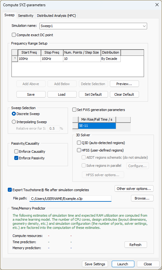
2. From the SIwave area, click Compute SYZ Parameters to open the Compute SYZ-parameters window.



3. From the Simulation Name field, enter a name for the solution.
4. If appropriate, check the Compute exact DC point check box to combine DC results with the frequency-swept AC results. This provides improved accuracy over the entire simulation bandwidth.
   Important:

   The Compute exact DC point and Enforce causality options are mutually exclusive. Selecting both generates an error.

5. For each frequency point in the Frequency Range Setup area, enter values for Start Freq. and Num. Points.
6. Use the Distribution drop-down menu to select a distribution method:
   • Linear – the difference between the start frequency and the stop frequency is calculated and is divided by the number of solution points.
   • By Decade – distributes the number of points specified logarithmically, over each decade.
7. Enter a value for either Stop Freq. or Min. Rise/Fall Time.
• The Min. Rise/Fall Time value represents the time scale that characterizes the rate of change of the input time signal that will be applied in the circuit simulator.
  Note:

  Entering data in one field automatically sets the other. The maximum frequency is considered to be the knee frequency, f_knee, which is related to the rise time T_R by the formula:

  f_knee = 0.5 / T_R

8. If appropriate, you can add or remove frequency points using the Add Above, Add Below, and Delete Selection buttons.
9. If appropriate, click Save to save frequency point settings as an SIwave Frequency Sweep Distribution File (*.sfsdf). To load previously saved settings from a *.sfsdf file, click Load.
10. If appropriate, click Set Default to make current settings the default for the simulation type. To return to the original default settings, click Clear Default.
11. If appropriate, click Preview to open the Frequency List Preview window.
12. From the Sweep Selection area, use the radio buttons to select either Discrete or Interpolating.
    • An interpolating sweep estimates a frequency response for an entire frequency range by solving at a relatively small number of frequency points within that range. Between the actual solution frequencies, the frequency response is obtained by rational interpolation. SIwave adaptively chooses the frequency points at which it computes the field solution. After a new frequency point is solved, a new interpolating fit is generated. This is compared to the interpolant from the previous step, and the maximum difference between the two is determined. If the difference exceeds the requested tolerance, then a new frequency point is chosen for a solution. The interpolating sweep is complete when the difference between successive interpolants is less than the error tolerance criterion.
    • If you choose Interpolating, you must also specify the error tolerance.
13. From the Passivity/Causality area, use the check boxes to Enforce Causality and/or Enforce Passivity.
    Important:

    The Compute exact DC point and Enforce causality options are mutually exclusive. Selecting both generates an error.

14. If appropriate, check Set FWS generation parameters to export the full-wave SPICE subcircuit.

The Start Frequency value changes to 0Hz. If you have an existing S-parameter solution, you can run an FWS simulation without needing a 0Hz or 1Hz point.

15. If appropriate, check Q3D (auto-detected regions) to utilize the Q3D solvers for 3D-type regions such as unreferenced traces, complex via transitions and pad coupling.
16. If appropriate, check HFSS (user-defined regions) to use the predefined HFSS regions and launch the HFSS simulation options. Click the HFSS solver options button to open the General tab in the Simulation Setup window, and set the solver options.

The following guidelines must be followed:

• You must manually define regions. Regions must contain signal net geometry that is included in the simulation. A region containing only power/ground net geometry or signal net geometry that is not included in the simulation is invalid.
• Ports must exist either completely inside or completely outside of a region. Simulation configurations consisting of ports that straddle regions are invalid.
• HFSS regions (which are user defined) and Q3D regions (determined by the solver) can coexist.
• Power/Ground nets should be properly classified.
• Signal net geometry in the region, along with power/ground net geometry, is solved using HFSS and the resulting S-parameters are incorporated into the SIwave solve to compute a unified channel response.
Note:

For both S-Parameter sweep and HFSS Regions simulations, the machines used are those specified in the Compute SYZ-parameters > Distributed Analysis tab. When multiple regions are present, the regions are solved sequentially, but the adaptive passes and frequency sweep within a given region are distributed.

The AEDT Regions Schematic check box allows you to export HFSS regions as a schematic without running a simulation.

The Solve Regions in Parallel check box allows you to configure HFSS region simulations in parallel.

17. If appropriate, check Export Touchstone file after simulation completes to automatically generate a Touchstone file (*.sNp, *.ts).
18. If appropriate, click Other solver options to open the SIwave Options window and further customize the simulation.
    Note:

    If the Time/Memory Predictor area does not appear on the Sweep tab, skip to step 20.

19. As explained in the following screenshot, the time/memory predictor estimates the length of time it will take to complete the simulation and the expected RAM use during the simulation, based on an internal Machine Learning (ML) algorithm. The predictor can estimate time and memory utilization of all SYZ simulations, excluding those that include HFSS and/or Q3D regions, or DC point simulations.
    Note:

    The Time/Memory Predictor is a feature available to Ansys AI+ license subscribers, and does not appear otherwise.

    From the Time/Memory Predictor area, click Refresh to populate the table with three rows of pertinent data.

    

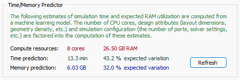
    • Computer resources – number of cores and memory allocated to the simulation (i.e., user-defined parameters selectable from the SIwave Options window > Multiprocessing tab).

    • Time prediction – time (in minutes) for the simulation to complete.

    • Memory prediction – allocated memory (in gigabytes) required for the simulation to complete.

    The second column in the Time/Memory prediction rows show the average expected variation in the accuracy of the predictions, based on the ML-algorithm.

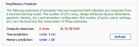
    Note:

    If the predictor determines that the time and/or memory allocation falls under the minimum threshold(s), then precise values and expected variation are not shown. Instead, the predictor will show Under 5 min and/or Under 1 GB, respectively.

    

20. Select the Sensitivity tab.

    

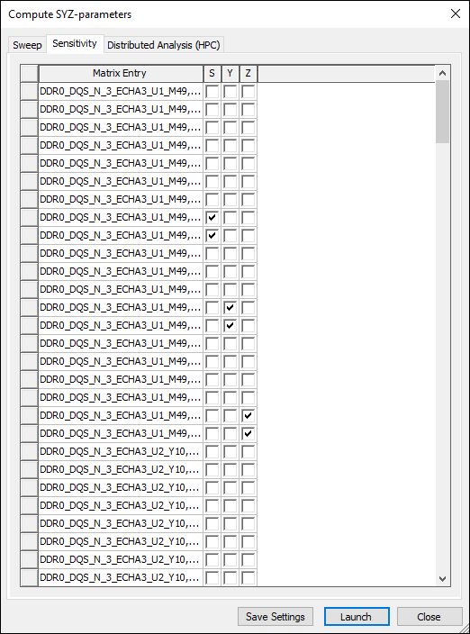
21. Select S, Y and Z parameters for the matrices. This computes the partial derivative of an entry of the S, Y or Z-parameter matrix with respect to the impedance of a circuit element.
22. Select the Distributed Analysis (HPC) tab to specify a distributed analysis over multiple machines.

    

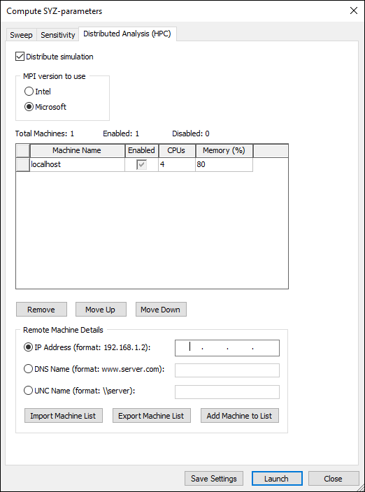
23. To enable distributed analysis, check the Distribute simulation check box.
24. From the MPI version to use area, use the radio buttons to select either Intel or Microsoft.
25. The list displays remote machines to be used in the simulation. You can Remove machines or rearrange them by clicking Move Up and Move Down.
26. To add a machine, enter its information in the Remote Machine Details area and click Add Machine to List.
27. To export the list as a *.txt file, click Export Machine List. Click Import Machine List to load a previously saved list.
28. If appropriate, click Save Settings to keep your settings for subsequent simulations.
29. Click Launch to run the simulation. The Messages window updates with a Process Monitor tab that displays the progress.