


After you have carefully inspected the available information, you can begin the actual troubleshooting work. The objective is to try to find a reasonable explanation for the non-convergence – and hopefully, also a remedy.
At this point, do not change the control card settings (keep them as shown in Table 5.1: Element Types for Nonlinear Implicit Analyses, other sources, or your private preferences). The many options and possible combinations of control card settings in LS-DYNA makes it tempting to modify them to obtain convergence or to assume that the convergence problem is caused by the control card settings. However, before making any modifications to the control card settings, it is strongly recommended to first investigate other possible reasons for the convergence problems.
A suggested action list [21] follows:
- 11.3.1. Perform a Basic Model Check
- 11.3.2. Check Model Connectivity
- 11.3.3. Check Element Connectivity
- 11.3.4. Avoid Release Conditions
- 11.3.5. Check Tied Contacts
- 11.3.6. Avoid Unintended Initial Penetrations in Contacts
- 11.3.7. Define Thickness Variation of Shell Parts
- 11.3.8. Use 2D Contacts in 2D Analyses
- 11.3.9. Check the Material Models
- 11.3.10. Examine the Deformation of a Non-converged State
- 11.3.11. Check if the Physical Problem is Unstable
- 11.3.12. Disregard Initial Geometric Stiffness
- 11.3.13. Switch to a Full Newton Solution
- 11.3.14. Activate Non-symmetrical Equation Solver
- 11.3.15. Check for "Too Easy" Convergence
- 11.3.16. Check Line Search History
- 11.3.17. Inspect Node IDs with Maximum Residuals
- 11.3.18. Use Sense Switch Controls
- 11.3.19. Convert to Explicit Analysis
- 11.3.20. Plot residual histories in LS-PrePost
If convergence problems persist, do not hesitate to contact your LS-DYNA supplier.
Perform a basic model check, as outlined in [24]. For example, you can use LS-PrePost ( > > > ).
Inspect the model carefully with respect to element quality, small (or even negative) initial volume of solid elements, and small Jacobian values.
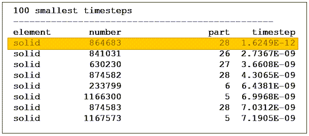
To some extent, the explicit time step listing in the d3hsp file can be used as an element quality indicator. For example, if the first listed element has an explicit time step which is several orders of magnitude lower than the others, it can be an indication that this is maybe an element which violates the quality criteria. The following figure shows an example of a time step that might indicate a problem with an element. Element number 864683 (highlighted in the following figure) has a time step that is about 1000 times smaller than the other elements. This indicates poor element quality.
The warning for a bad Jacobian, for example:
 *** Warning solid element # XX has a bad jacobian
                        value -3.991E-01
is in general an indication that re-meshing is required.
Starting at R14, lists of shells and solid elements with the worst aspect ratio are printed. Search for "Listing the top" in the d3hsp file. Also, a check for elements with nearly coincident nodes is added, for example:
 *** Warning 60421 (IMP+421)
Solid element XX has a slightly bad edge/diag ratio,
check if nodes are coincidental and adjust mesh.
or in more severe cases, the warning:
 *** Level3-Warning 60421 (IMP+421)
Solid element XX has a fatally bad edge/diag ratio,
check if nodes are coincidental and adjust mesh.
Check that no unintended cracks in the mesh are present.
Check that consistent units are used for materials, loadings, accelerations, time etc.
Check for duplicate elements, needle elements, and so forth.
Split any pyramid elements to tetras. There is no proper pyramid element in LS-DYNA.
Delete free, unreferenced nodes from the model.
Check the model connectivity. Unconnected sub-assemblies or "loose parts" cause rigid body modes in implicit statics, potentially causing convergence problems. One indication of this problem is negative eigenvalue warnings like the following in the d3hsp file.
 *** Warning 60124 (IMP+124)
 XX negative eigenvalues detected
Unintentionally loose sub-assemblies that start to spin can cause slow convergence in implicit dynamics. Ways of checking model connectivity are:
Perform an eigenvalue analysis, (
*CONTROL_IMPLICT_EIGENVALUE), see Eigenfrequency Analysis. Inspecting the obtained d3eigv file usually reveals rigid body modes or mechanisms in a very efficient and visual way.By inspecting the d3iter files using LS-PrePost, rigid body modes or parts "flying away" can also be identified.
Some preprocessors have dedicated functionality for detecting unconnected assemblies, based on contacts and connectors defined in the model.
In many analyses, the presence of rigid body modes is intentional. A typical example of this is an assembly that is to be connected via bolts and contacts. Before the bolt pretension is applied, such an assembly has many rigid body modes [22]. Set IMASS = 1 on *CONTROL_IMPLICIT_DYNAMICS to activate implicit
dynamics, at least during the initial phase, until contacts are fully established. This normally solves convergence problems due to intentional rigid body modes (see Bolt Pretensioning). In some cases, inertia relief boundary conditions (applied by *CONTROL_IMPLICIT_INERTIA_RELIEF) are relevant for handling intentional rigid body modes. In cases where
the rigid body modes are unintentional, due to forgotten boundary conditions, for example, simply apply the appropriate boundary conditions.
Verify that the element connectivity is valid. Be cautious when continuum elements (typically solids) and structural elements (beams, shells) share nodes. Invalid connectivity can cause unintended hinges, joints, or other mechanisms. For example, connecting a beam element between two solids using only shared nodes leaves the possibility for the beam to spin freely around its axis. Connecting shells to solids along a single row of nodes could create a hinge. In some cases, the program issues warning messages for potentially problematic connectivity, for example:
 *** Warning 60301 (IMP+301)
Using *CONSTRAINED_SPOTWELD with nodes without rotational dofs.Avoid the use of release conditions on constrained nodal rigid bodies (CNRBs). It is not recommended to use DRFLAG,RRFLAG ≠ 0 on CNRBs (other than for two-noded CNRBs in linear implicit analyses, NSOLVR = ±1 on
*CONTROL_IMPLICIT_SOLUTION). If release of degrees of freedom is required, use joints (*CONSTRAINED_JOINT_...) instead.
From R11 of LS-DYNA, joint stiffness and damping can be applied globally on
*CONTROL_RIGID by the variables
GJADSTF,GJADVSC,
TJADST and TJADVSC. This
allows for the addition of a small artificial stiffness to improve convergence of
models with numerous joint definitions.
As a troubleshooting step, disable joint failure (switch
*CONSTRAINED_JOINT_{) at least in the
initial model development phase.TYPE}_FAILURE to
*CONSTRAINED_JOINT_{TYPE}
Check tied contacts. This is often closely related to the model connectivity since tied contacts are often used for assembling different parts or sub-assemblies of a model.
Most preprocessors have built-in tools for checking tied contacts, for example in LS-PrePost, it is accessed via > > > > ).
Ensure that the intended tracked nodes are properly tied. Too many ties can cause surprisingly rigid behaviour while too few can lead to unintended rigid body modes.
*CONTACT_TIED_...reports nodes that are not tied to the d3hsp file. The result can be visualized in LS-PrePost using > (or similar functionality in other preprocessors).Non-offset tied contacts (see Table 6.1: Overview of some tied contact options) moves the tracked nodes to the reference segments. In some cases, this can cause mesh distortions, especially if a large search distance is given. Look for:
*** Warning 41240 (SOL+1240)
The remedy for this may be to switch to an offset tied contact or reduce the search distance.
If 2nd order elements are involved in a tied contact, use a node set (including mid-side nodes) on the tracked side and define the reference side by part ID or part set ID (
SURFBTYP= 2 or 3).If structural elements (shells, beams, … or nodes of these element types) are involved in a tied contact, use
*CONTACT_TIED_SHELL_EDGE_TO_SURFACE_{in order to avoid spinning beams or hinges in the model.OPTION}
Using a tracked node set gives better control over the possible tied nodes than if
a tracked part set is used. The tie distance can be manually adjusted as described
in Tied Contacts. When using constraint-based tied contact,
nodes subjected to other constraints (*CONSTRAINED_NODAL_RIGID_BODY,
*BOUNDARY_SPC, ...) cannot be tied. One remedy may be to set
IPBACK > 0 on Optional Card E of the
*CONTACT_TIED_ definition. The program automatically creates a
penalty-based tied contact for nodes that are subjected to other constraints.
Avoid unintended initial penetrations in contacts. The
IGNORE = 2 option of Mortar contacts can handle
"reasonably large" initial penetrations, but a penetration free initial
configuration is always preferred.
Most preprocessors have built-in tools for checking and correcting initial penetrations, for example LS-PrePost accessed via > > > > .
Mortar contacts report initial penetrations in the mes0* files. Look for:
Mortar contact information for contact ID …
This information can be used to verify that the contact penetration checks of the preprocessors agree with how LS-DYNA interprets the initial contact state.
Initial penetrations may be reported in the d3hsp or
mes0* files but not be found in the preprocessor (refer to
the figure below for an example). To fix this, specify a reasonably small "contact
thickness" for solids using the PENMAX parameter (compare
Figure 6.1: Using PENMAX to define the contact thickness for
solid parts.).
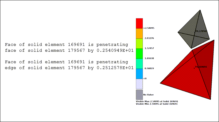
The left side of the image above shows an extract from the d3hsp file where the elements are reported as penetrating, even though they are clearly separated, as shown in the illustration on the right.
From R12 of LS-DYNA, penetration information can also be visualized (fringe
plotted) from the d3plot file by setting
PENOUT = 1 or 2 on
*CONTROL_OUTPUT.
When you know beforehand that no self-contact within the same part occurs and a
single surface Mortar contact is used for convenience, the option
IGNORE = -2 can improve convergence by neglecting
self-contact within the same part, avoiding spurious self-contact.
Use IGNORE = 3 or 4 of the Mortar contact [23] to resolve press-fits or other intended initial penetrations.
When shell parts with varying thickness are involved in Mortar contacts, it is
often beneficial for convergence to define the thickness variation by
*ELEMENT_SHELL_THICKNESS rather than splitting up a (physical) part
into many different parts with the thickness variation defined by different
*SECTION_SHELL.
For 2D analyses, use the appropriate 2D contacts, see Contacts for 2D Analyses.
Check the material models.
Avoid using
*MAT_ELASTICwith n » 0.5 for modelling rubber, at least for finite deformations. Instead, use*MAT_HYPERELASTIC_RUBBERor*MAT_SIMPLIFIED_RUBBER_FOAM(see Rubber Modeling for Implicit Analysis).If a simple elastic-plastic material model with isotropic hardening is desired, use
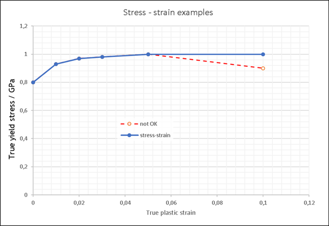
*MAT_PIECEWISE_LINEAR_PLASTICITYrather than setting BETA = 1 for*MAT_PLASTIC_KINEMATIC.Inspect hardening curves and avoid a negative slope in the last segment of the curve. LS-DYNA extrapolates the hardening curve based on the slope of the last segment, which can result in negative yield stress values and prevent convergence.
Figure 11.8: Example of hardening curves - avoid a negative slope for the last segment (dashed red line)
Note: Some material models are not supported for implicit analyses.
To troubleshooting an unconverged analysis, you can be to switch all material models to
*MAT_ELASTICwith sensible parameters and rerun the simulation. If convergence improves, this may indicate that the problem is related to the original material models. In some cases, switching material models may result in a simulation that can proceed a bit further, perhaps revealing other problems with the model.Avoid involving parts with
*MAT_NULLin tied contacts.If
*MAT_NONLINEAR_ELASTIC_DISCRETE_BEAM (*MAT_067)is used in the model, and you suspect that it may cause convergence problems, try switching to*ELEMENT_DISCRETEwith*MAT_SPRING_NONLINEAR_ELASTIC (*MAT_S04).Starting at R11 of LS-DYNA, material models
MAT_24andMAT_123are more tightly integrated with the nonlinear implicit solver. These material routines can cause a retry of an implicit time step if the increment of plastic strain is too big. This triggers the following message in the d3hsp file:Material model rejected current iterate, list of elements affected follows (at most 20): Element # 1234
This could indicate a problematic area of the model. Inspect the model using the d3iter and d3plot files, in the vicinity of the listed elements (1234 in the above example).
Inspect the material model and doublecheck units, hardening curves, and so forth.
The message may simply indicate that the time step used was too big, and should in those cases not be seen as too alarming.
If the rejection occurs frequently, try switching from
MAT_24toMAT_103 (*MAT_ANISOTROPIC_VISCOPLASTIC, see Material Models)From version R16 of the Ansys LS-DYNA software, you can disable material rejection by using the settings of
*CONTROL_MAT:*CONTROL_MAT $# maef - umchk oldint noreject 1You can disable material rejection as part of the troubleshooting process. Switch material models or use the previous
*CONTROL_MAToption from R16. If your results are acceptable with respect to solution quality (force and energy balance, and so forth) this technique can also help you to solve convergence problems.
The d3iter file provides useful visual information that indicates reasons for the convergence problems. For example, looking at the deformation of a non-converged state shows whether loose parts "fly away" due to rigid body modes.
Scale up the displacement or look at a fringe plot to identify areas of the model where large changes in displacement take place between iterations. This highlights problematic areas of the model.
Extreme deformations may be an indication that inconsistent units are used.
By setting
RESPLT= 1 on Card 4 of*DATABASE_EXTENT_BINARY, you can create a fringe plot of the force residual from the d3iter binary database. This can also be useful for pinpointing the areas of the model where convergence is the most challenging.
Is the physical problem itself unstable? Does collapse, buckling, or bifurcation occur? If the applied loading exceeds the ultimate capacity of a structure, convergence in implicit statics is, in practice, impossible to reach.
Try switching from load to displacement control (see Figure 8.1: Example of different load application approaches. ).
Activate the arc-length solver (see Nonlinear Analysis Using the Arc-length Method)
Activate implicit dynamics (see Nonlinear Implicit Dynamic Analysis). Note that in implicit dynamics, time means physical time. If, for example, the unit system kg-mm-ms is used, an appropriate load application time would be on the order of 1000 ms.
For analyses involving rubber (or other incompressible materials), try disregarding the initial geometric stiffness effect by setting IGS = 2 on *CONTROL_IMPLICIT_GENERAL.
Disabling the geometrical stiffness can improve convergence in other situations. It is disabled in the control card files provided with this guide in Example Files for Implicit Analyses.
Negative eigenvalue warnings that cannot be related to rigid body modes or mechanisms are probably due to severe deformations of the elements. In such situations, you can use under-integrated elements (solid element formulation 1) or CPE elements, activated by choosing Hourglass formulation 10 for solid element formulation 1 or 16.
In some cases of extreme deformation of shell structures, you can activate the hourglass type 8 for shells of element formulation 16 as shown in Figure 5.1: Crash box compression analysis.
Switching to a full Newton solution scheme can be efficient for solving highly nonlinear problems. This means that the stiffness matrix is reformulated and factorized for each iteration.
If the default BFGS method consistently requires very many (>100) iterations to converge, or if the residual norms decrease very slowly with each iteration, it may be in place to switch to full Newton.
Set ILIMIT = 1 and increase MAXREF to 30-60 on
*CONTROL_IMPLICIT_SOLUTIONto activate a full Newton solution.The settings of
*CONTROL_IMPLICIT_AUTOmay have to be adjusted to account for the reduced number of total iterations allowed.
Activating the non-symmetrical equation solver can improve convergence in some cases, for example follower loads, "snap-through" deformation, or contacts with high (µ ≈ 0.3 or above) friction. It can also prove convergence for cases involving anisotropic material models.
Set LCPACK = 3 on
*CONTROL_IMPLICIT_SOLVER.
Check for "too easy" convergence. This means that LS-DYNA has previously accepted a state even though it was not converged "enough" (that is, some residual forces or deformations remain in parts of the model). When proceeding from this state, the residuals might lead to non-convergence, since the problems from previous steps remain unresolved.
Check for "noisy" contact force histories or unsatisfied global equilibrium (for example if spcforc does not add up to the external forces) or large force residuals are printed in the d3hsp file.
To remedy this, try tightening the tolerances slightly on
*CONTROL_IMPLICIT_SOLUTION, for example by settingDCTOL= 5E-4 and/or adding residual force criterionRCTOL≈ 0.02 - 0.1.
Some clues may be found by tracking the convergence information regarding the line search history, see Figure 11.1: Tracking convergence information in the mes0* files. Typically, the line search should converge within 10 iterations. If the line search requires significantly more than 10 iterations to converge and the residuals remain high even with very small step sizes, nonconvergence may be due to severe overloading of the structure. In such cases, check that consistent units are used and the loading has the correct order of magnitude. If the loading is correct, it might help to reduce the time-step size.
Note that the node ID/rigid body ID with the maximum residuals are listed in the iteration information (see Figure 11.1: Tracking convergence information in the mes0* files). Inspecting the model at these ID:s and perhaps, their surroundings might provide insight about what is causing the convergence problems. This can be, for example, poor element quality or unconnected parts. This is especially likely if the same ID:s show up as critical for several consecutive iterations. These entities can be highlighted on the model using the D3hsp View tool, see Figure 11.5: The D3hsp view-tool in LS-PrePost and by tracking the convergence histories, as shown below.
For extended interactive troubleshooting, you can send sense switch controls to the Ansys LS-DYNA software. Create a text file named d3kil in the directory where the current simulation is running. The text file should contain one of the following text strings to control the implicit analysis:
convForces implicit nonlinear convergence for the current time step.
ttrmTerminates iterations for the implicit time step, then retries the time step with a reduced time increment.
rtrmTerminates implicit analysis at the end of the current time step.
lpriToggles implicit linear algebra solver output on or off.
nlprToggles implicit nonlinear solver output on or off.
IterToggles implicit output to the d3iter database on or off.
convForces the current time step to converge and pushes the solution one step further. This can help you to gather information from the evolution of the solution and discover more clues about why your soution is not converging.
Important: The sense switch
convis intended only for troubleshooting. Do not use it as part of a permanent solution.
For more information on using sense switch controls, see the Getting Started section of Keyword Manual Vol. I.
Converting the model for explicit analysis (see Converting an Implicit Model for Explicit Analyses for details) can give valuable insight for troubleshooting (such as unconnected parts "flying away").
In cases when convergence cannot be obtained using the implicit solver, switching to explicit analysis is an alternative option for obtaining a solution.
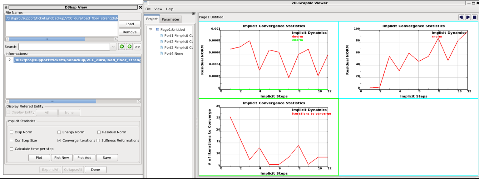
Residual histories, iterations to converge, etc. may also be plotted in LS-PrePost (starting at version 4.5) using >, see Figure 11.9: Tracking the convergence histories using the D3hsp View tool in LS-PrePost.