Eigenfrequency analysis is a way of determining the fundamental frequencies and shapes of harmonic vibration of a system. The equations of unforced motion can be put as

By the ansatz , the generalized eigenvalue problem

is obtained, with the eigenfrequency .

You can use eigenfrequency analysis to verify that the eigenfrequencies of the system do not coincide with critical excitation frequencies. You can also use it as a tool for checking model integrity, as mechanisms and rigid body modes are effectively revealed. Another common use for eigenfrequency analysis is to calculate a modal basis for further dynamic analyses (see Linear Transient Modal Dynamic Analysis and Frequency Domain Analyses).

To activate eigenfrequency analysis, use the keyword *CONTROL_IMPLICIT_EIGENVALUE. Intermittent eigenfrequency analyses are also possible as a part of a linear or nonlinear analysis [4]. This means that the effect of loading (such as bolt pretensioning) on the eigenfrequencies can be accounted for. See the example in Intermittent Eigenfrequency Analysis of a Bolted L-bracket.

To compute modal stresses, set the parameter MSTRES = 1. This is required if strain energy density is to be evaluated, as described in Visualization of Strain Energy and Strain Energy Density. If the computed eigenvectors are to be used as a modal basis in a frequency domain analysis where stress evaluations are of interest, see Frequency Domain Analyses.

Use non-Mortar sliding contacts with care in an eigenfrequency analysis. See Sliding Contacts in Eigenvalue Analyses and Linear Implicit Analyses.

A template for eigenfrequency analyses follows:

*KEYWORD
.
.
.
*INCLUDE
database_cards_static.key
*CONTROL_TERMINATION
            Define end time of the simulation
*CONTROL_IMPLICIT_EIGENVALUE
            Card 1: Define number of eigenmodes, frequencies etc.
            Card 2: Set MSTRES=1 to request modal stresses
*INCLUDE
            Include file defining geometry, materials etc.
*LOAD_...
            Define nodal loads etc.
*BOUNDARY_...
            Data line to prescribe boundary conditions
*TITLE
            Simulation title
*END

A basic eigenfrequency example is presented in Eigenfrequency Analysis of a Panel With a Bead.

By default, the eigenfrequency analysis is performed at the beginning of the simulation, which then terminates. It is possible to perform intermittent eigenfrequency analyses at different stages of the simulation. A curve ID can be specified by entering the LCID as a negative number. The x-values of the curve specify at which time(s) the eigenfrequency analyses are to be performed. The corresponding y-values specify the number of eigenmodes to compute. When performing intermittent eigenfrequency analyses, keypoints corresponding to the times for the eigenfrequency analysis must be added to the synchronization curve (LCID 700, see the plot in Figure 4.5: Using the time incrementation curve to synchronize the simulation with applied loading). See also the example Intermittent Eigenfrequency Analysis of a Bolted L-bracket.

The multistage approach is another option for performing intermittent eigenvalue analyses, as described in Combining dynain.lsda and *CASE for Multistage Analyses and Appendix X of Keyword Manual Vol. I.

The eigenfrequencies are printed in the eigout file. The database for visualizing modal deformations (eigenvectors) is called d3eigv. Eigenvectors in LS-DYNA are mass normalized, which implies that

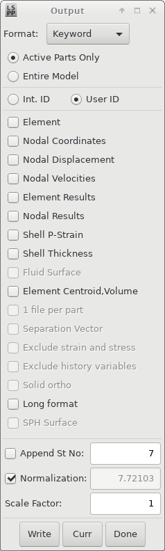
The eigenvectors are rescaled for improved visibility when they are output in the d3eigv file(s). The scale factor can be obtained from LS-PrePost as described in the following procedure. In versions starting with R12.2, the scale factors are also printed in the eigout file (search for "EIGENVECTOR SCALING FACTOR".)

In LS-PrePost:

Figure 4.17: Output of scale factor for mode shapes from LS-PrePost.

Another option for obtaining the unscaled eigenvectors is to use the functionality for dynamic condensation and superelement creation of the keyword *CONTROL_IMLPICIT_MODES. This keyword outputs the unscaled eigenvectors to the d3mode binary database in addition to the d3eigv files. The d3mode file(s) can be opened in LS-PrePost for 3D visualization and postprocessing.

If the d3eigv files are to be used in mode-based analyses (seeLinear Transient Modal Dynamic Analysis and Frequency Domain Analyses) they must be in double precision format for all mode-based analyses. Do not use *DATABASE_FORMAT to request single precision output in this case.

The default solution method for eigenvalue problems in LS-DYNA is block-shift invert Lanczos. This is normally a fast and efficient method, especially in MPP. Since R11.1, the MCMS method is available in SMP [20] for computing many (>1000) eigenvalues of large models (> 1E6 elements). This is activated by setting EIGMTH = 101 on card 1 of *CONTROL_IMPLICIT_EIGENVALUE.

If only a few (< 50) eigenvalues of a large model are to be determined, the LOBPCG method may be of interest. It can be activated by setting EIGMTH = 102. The LOBPCG is only available in SMP in versions prior to R14, but an MPP implementation is also available from R14.

 

4.6.1. Visualization of Strain Energy and Strain Energy Density

Strain energy and strain energy density are commonly used measures for indicating the areas of the structure that are under the greatest stress and contribute most to the stiffness for a particular mode. You must request the output of modal stresses by setting MSTRES = 1.

LS-PrePost and some third party post-processors can be used to visualize the strain energy and strain energy density from the d3eigv file. (For additional required output settings, Ansys assumes that the control and database card settings provided in this guide are used, for example control_cards_linear.key and database_cards_static.key). This visualization is shown in the following figure. The strain energy is not computed by the LS-DYNA solver but is calculated as a postprocessing result by the postprocessing software.

Figure 4.18: Example of visualization of strain energy using LS-PrePost.

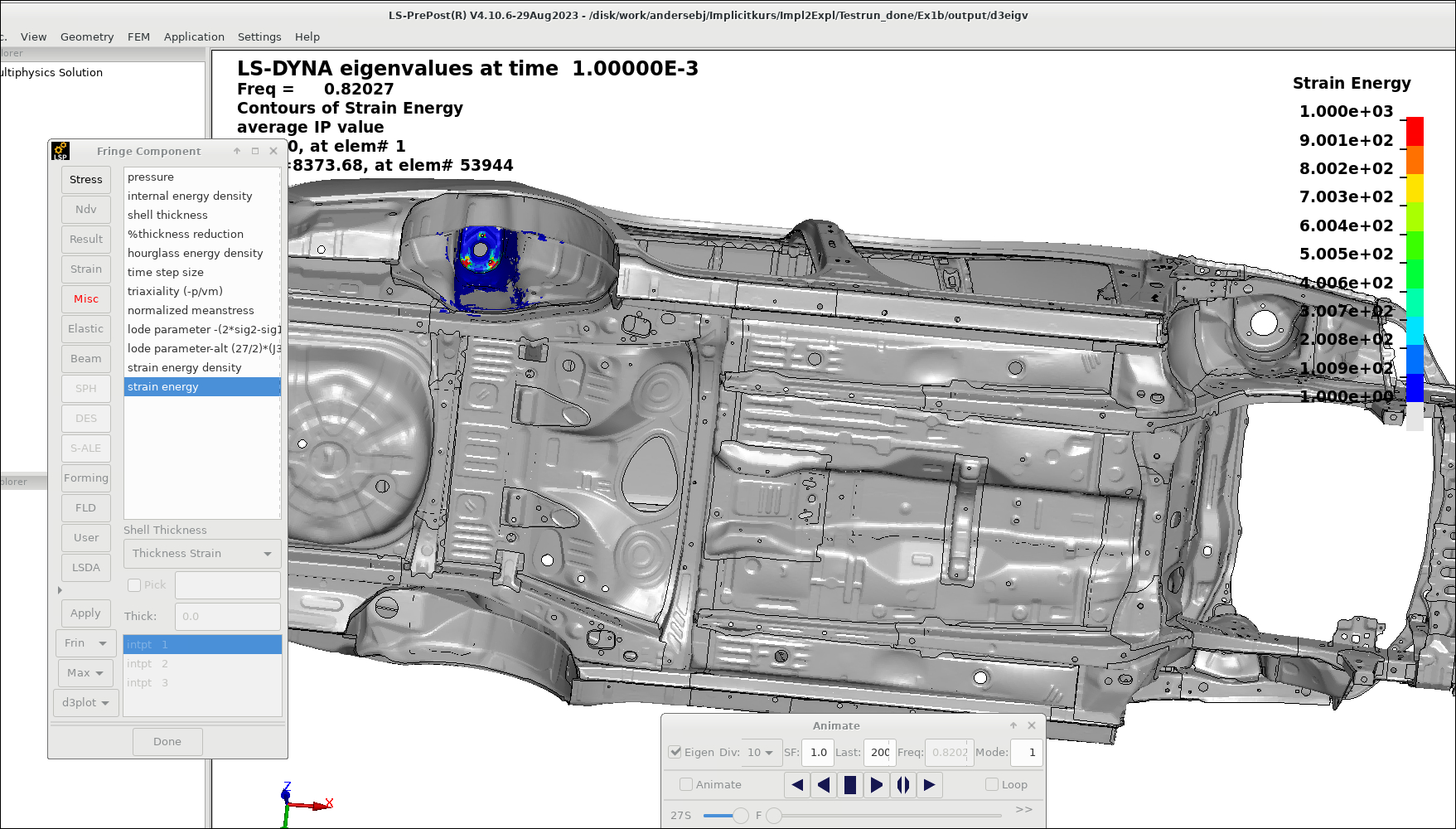
The model in the above figure [45] is courtesy of NCAC. The work of the Center for Collision Safety and Analysis at the George Mason University is gratefully acknowledged.

 

4.6.2. Eigenfrequency Analysis of a Panel With a Bead

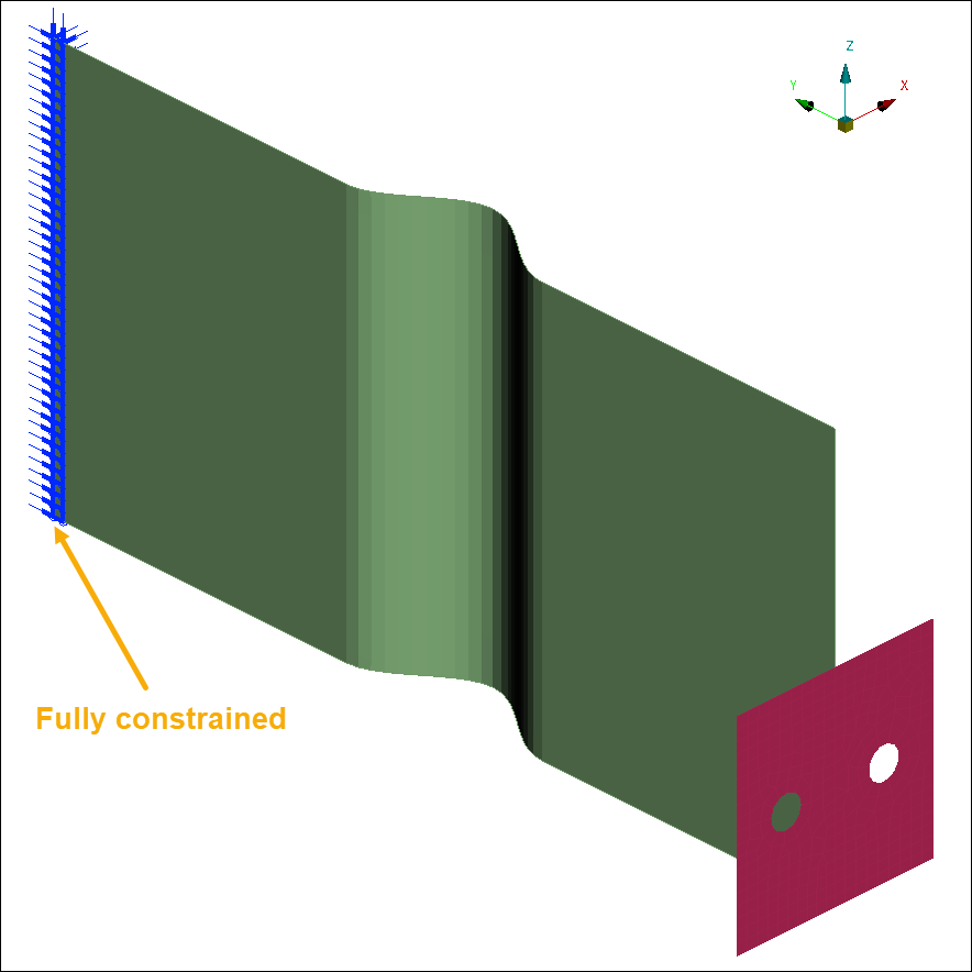
A panel is fully constrained at one edge as shown in the following figure. The example keyword file is eigen001.key. The lowest eigenfrequency is 44.3 Hz, and the mode shape is a side-to-side swinging motion.

Figure 4.19: Eigenfrequency analysis of a panel with a bead.