


Fully nonlinear static analysis is the default in LS-DYNA implicit analyses, including large strains and deformations. Sources of nonlinearity in a static analysis include the following:
nonlinear material models (plasticity)
contact,
large deformations,
nonlinear constraints (such as joints),
nonlinear loading (such as follower forces, where the force direction is defined relative to the deformed geometry), or
stress stiffening (guitar string effect).
An implicit analysis is either fully nonlinear or fully linear. From R15, the option to perform a linear analysis considering nonlinear contacts (see Linear Analysis with Nonlinear Contact) was added.
The keyword file control_cards_nonlin.key contains control card settings that are generally well suited for nonlinear static analyses. The automatic time incrementation is controlled by the load curve with ID 700, which you must define. The purpose of the load curve is as follows:
to define the maximum allowed time increment during the simulation. Reducing the time increment can aid convergence, if substantial nonlinearities are present in the model.
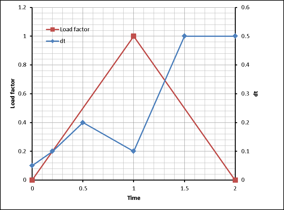
to synchronize the simulation time with the loading: at each time specified in the load curve ID 700, a converged step is obtained. See Figure 4.5: Using the time incrementation curve to synchronize the simulation with applied loading.
A template for a nonlinear static analysis follows:
*KEYWORD
*INCLUDE
control_cards_nonlin.key
*DEFINE_CURVE_TITLE
Implicit time incrementation
700,
0., dt0 (first timestep)
Additional lines to define time incrementation and synchronization with
      loadings
*INCLUDE
database_cards_static.key
*CONTROL_TERMINATION
Define end time of the simulation
*INCLUDE
Include file defining geometry, materials etc.
*LOAD_...
define nodal loads etc.
*BOUNDARY_...
Data line to prescribe boundary conditions
*TITLE
Simulation title
*END
For a static implicit analysis to converge, no rigid body modes or mechanisms can exist in the model. This means that you must provide sufficient boundary conditions in order to prevent rigid body motion of any part. Inertia relief boundary conditions can also be applied to nonlinear analyses. For further discussion, see Loads and Boundary Conditions.
Many analyses involve an initial stage where rigid body modes exist in the assembly.
These modes are eliminated when the parts come into contact, such as parts that are kept
together by bolt pretensioning. This situation can be handled by performing the initial
stage (for example, until contacts are established) using implicit dynamics
(*CONTROL_IMPLICIT_DYNAMICS, set IMASS = 1). For
more information, see Bolt Pretensioning.
The following figure shows the use of the time incrementation curve (blue) to synchronize the simulation with the applied loading (red curve). By specifying a value of (1.0, 0.2) for the time incrementation curve, a step at t = 1.0 (coincident with the maximum loading) is obtained.
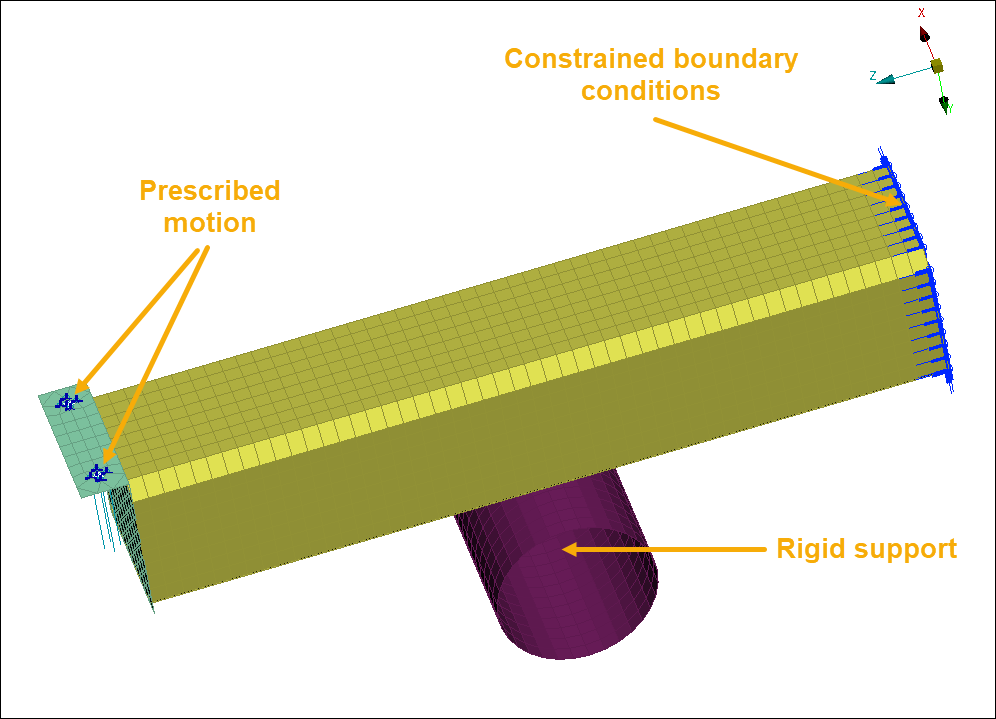
An aluminium cantilever beam is bent over a rigid support. The geometry for the example is shown in the following figure. At one end, the beam (yellow) is fully constrained (blue lines) while at the other end, a prescribed displacement is applied. nonlinear material properties are used in the beam. The contact between the beam and the support is modeled using
*CONTACT_AUTOMATIC_SURFACE_TO_SURFACE_MORTAR, see Contacts for Implicit Analyses. The example keyword file is bend001.key.
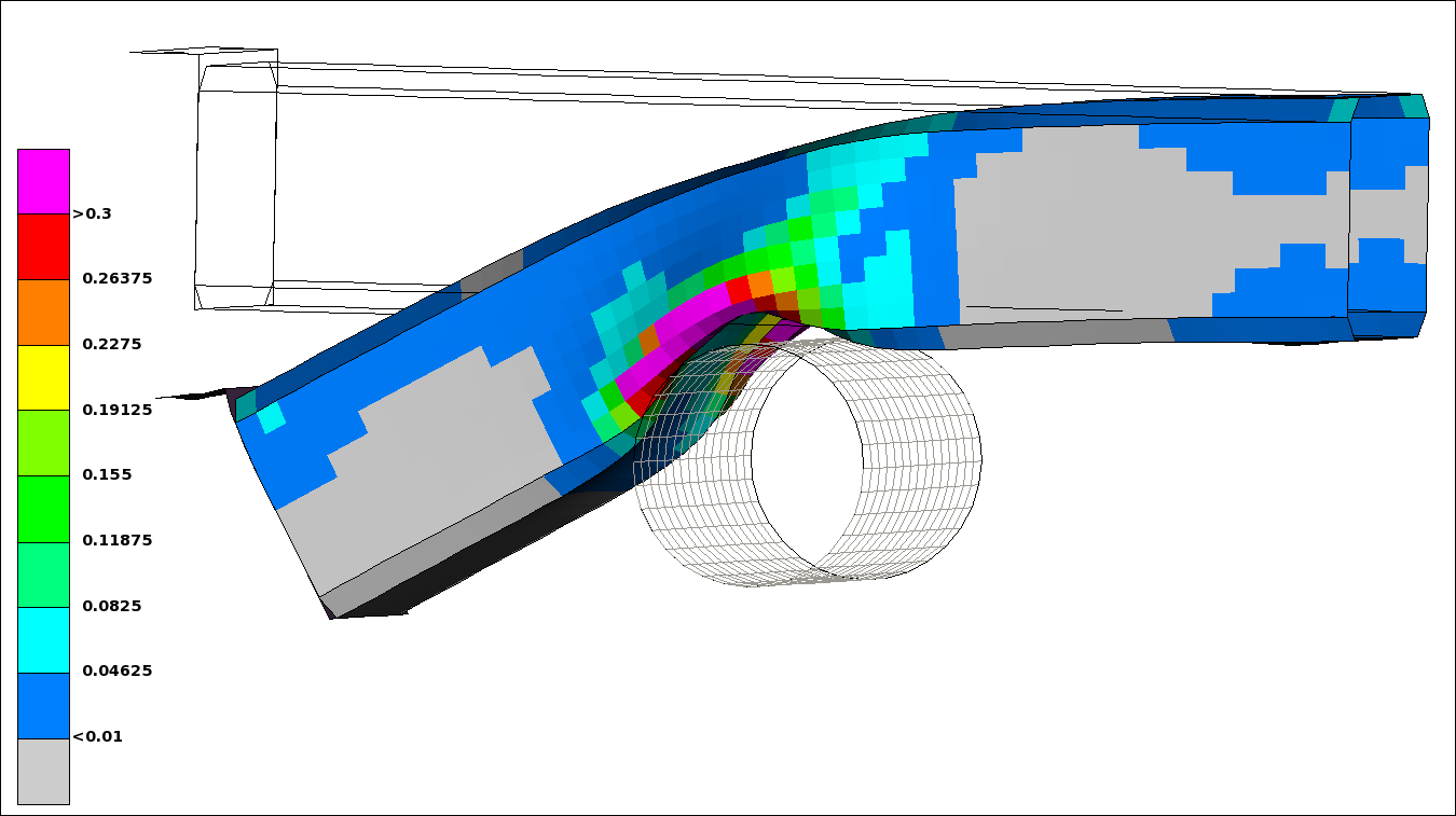
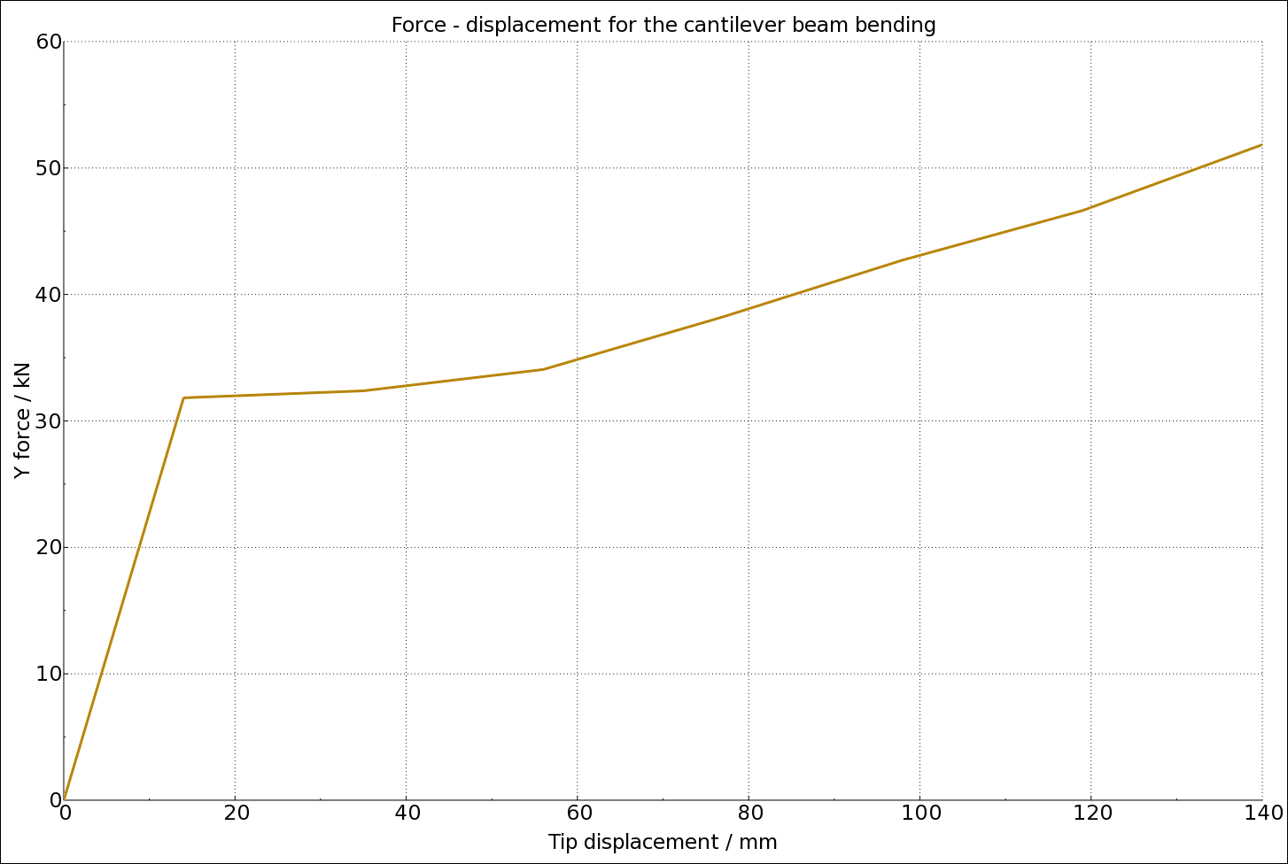
The results are shown in the following figures.
A version that uses a less strict convergence criterium is available in bend002.key. It sets DNORM = 2 on *CONTROL_IMPLICIT_SOLUTION. See Modifying Control Card Settings and Some Comments on Control Card Settings.
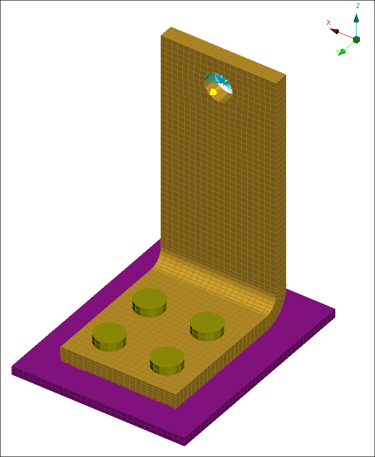
A bracket is connected to a base plate by four bolts, as shown in the following figure. A force (shown as a yellow arrow) is applied by a distributing coupling at the center of the hole in the flange.
The following figure shows the final state of the geometry and displays a fringe plot of von Mises effective stress.
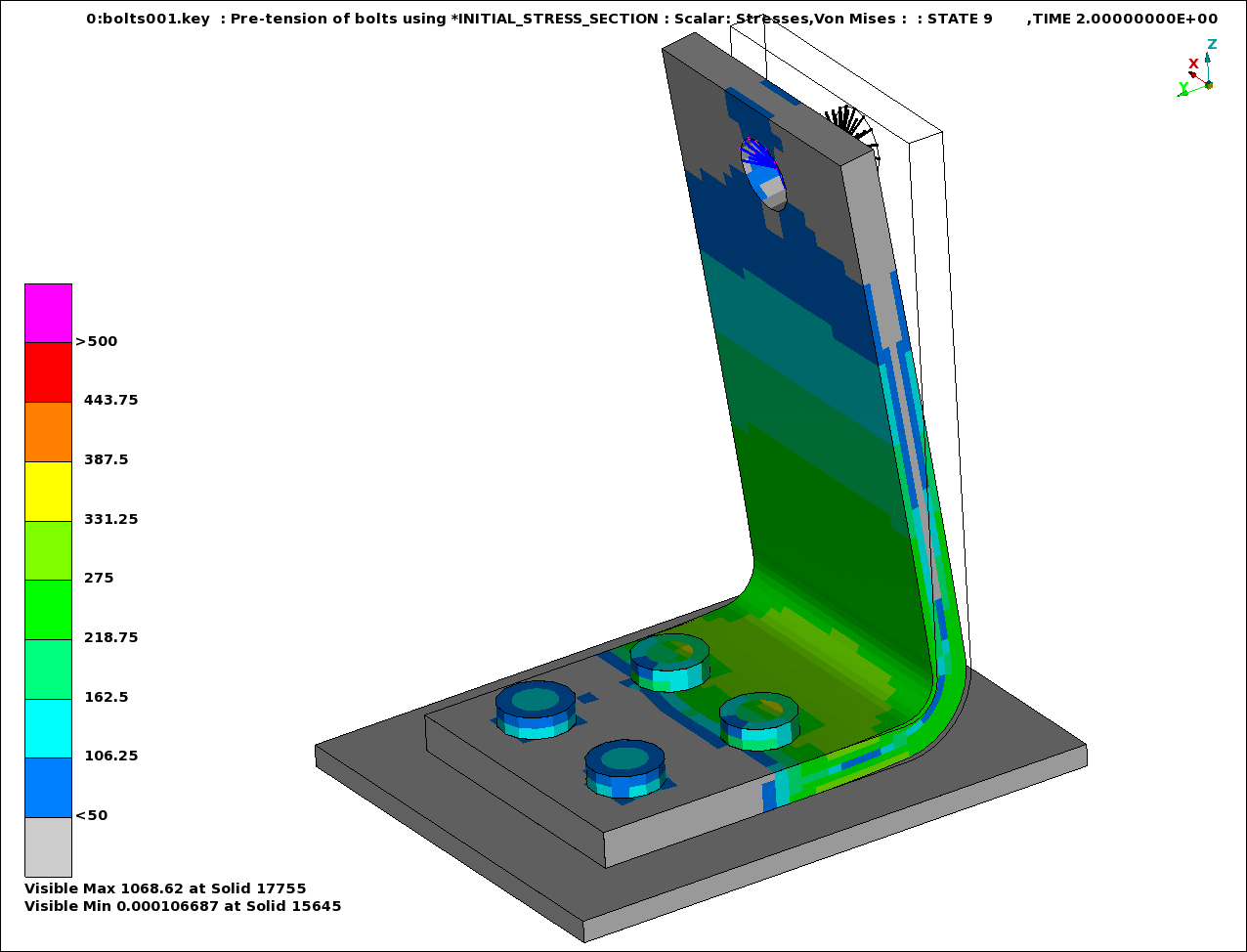
Bolt pretensioning is performed between t = 0 and t = 1. The keyword *INITIAL_STRESS_SECTION is used to apply the bolt pretensioning. From t = 1 to t = 2, a load is applied at the free hole of the flange via a distributing coupling (*CONSTRAINED_INTERPOLATION). The example keyword file is bolts001.key.
Implicit dynamics is used during the bolt pretensioning to overcome the fact that the model initially contains rigid body modes. A template for using implicit dynamics for this purpose follows:
*KEYWORD
*INCLUDE
control_cards_nonlin.key
*DEFINE_CURVE_TITLE
Implicit time incrementation
700,
0., dt0 (first timestep)
Additional lines to define time incrementation
*CONTROL_IMPLICIT_DYNAMICS
1, GAMMA, BETA, 0., TDYDTH, TDYBUR, IRATE
*INCLUDE
database_cards_static.key
*CONTROL_TERMINATION
Define end time of the simulation
*INCLUDE
Include file defining geometry, materials etc.
*LOAD_...
Define nodal loads etc.
*BOUNDARY_...
Data line to prescribe boundary conditions
*TITLE
Simulation title
*END
The parameters GAMMA and BETA of the
*CONTROL_IMPLICIT_DYNAMICS keyword (described in Nonlinear Implicit Dynamic Analysis) control the time integration. Normally
GAMMA = 0.6 and BETA = 0.38 are used
in order to introduce some numerical damping, when the purpose is to use implicit
dynamics in a (quasi) static analysis to resolve initial rigid body modes.
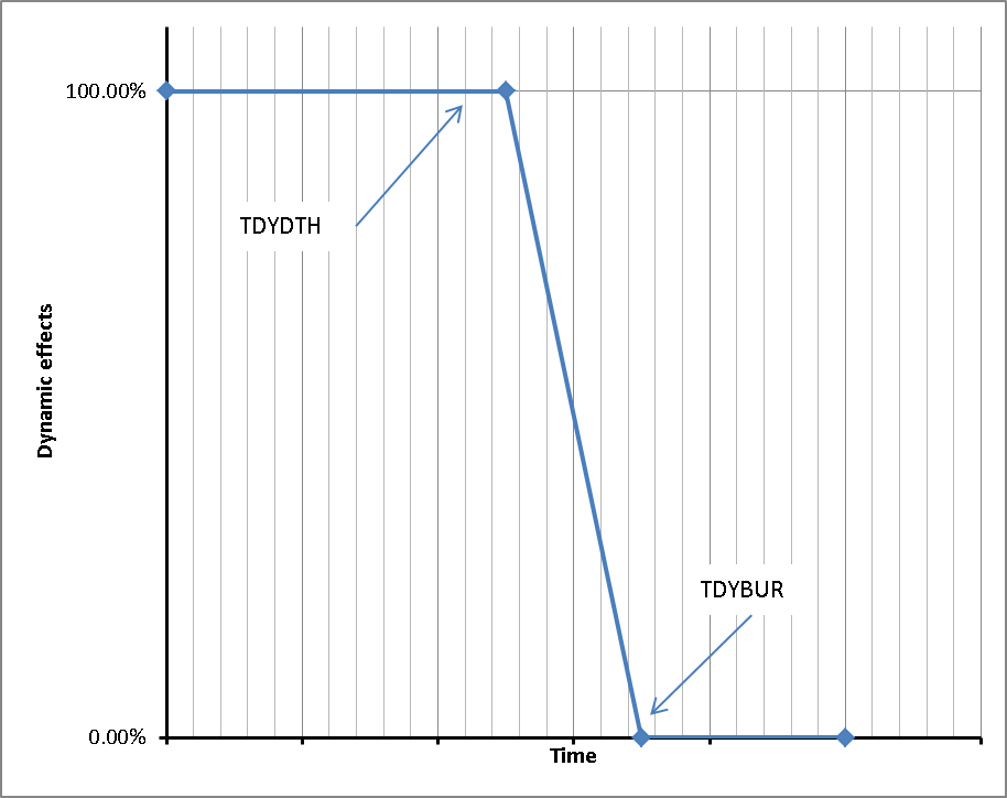
The parameter TDYDTH is the time when the dynamic effects start to ramp off, and at time TDYBUR the dynamic effects are completely removed as shown in the following figure. Setting the parameter IRATE = 1 will switch off the rate effects in material models, see Material Models.
See Bolt Pretensioning by Explicit Dynamic Relaxation for a slightly modified version of this example. Bolt pretensioning in LS-DYNA in general is discussed in [17], [29], [33], and LSDYNA Bolts (ansys.com)