Fully nonlinear implicit dynamics (including contacts, material nonlinearities and
large deformations) is activated by using the keyword
*CONTROL_IMPLICIT_DYNAMICS. The main purpose is to perform fully
nonlinear, transient dynamic analyses. However, this procedure can be used for the
initial phase of analyses of assemblies with "loose" parts (such as a bolted joint), as
described in Bolt Pretensioning.
A template for using implicit dynamics follows:
*KEYWORD
*INCLUDE
control_cards_nonlin.key
*DEFINE_CURVE_TITLE
Implicit time incrementation
700,
0., dt0 (first timestep)
            Additional lines to define time incrementation
*CONTROL_IMPLICIT_DYNAMICS
1, GAMMA, BETA, , , , , ALPHA
*INCLUDE
database_cards_dynamic.key
*CONTROL_TERMINATION
            Define end time of the simulation
*INCLUDE
            Include file defining geometry, materials etc.
*LOAD_...
            Define nodal loads etc.
*BOUNDARY_...
            Data line to prescribe boundary conditions
*TITLE
            Simulation title
*END
The parameters GAMMA and BETA of the
*CONTROL_IMPLICIT_DYNAMICS keyword control the time integration and the
amount of numerical damping that is introduced by the implicit time-integration scheme.
The default values are GAMMA = 0.5 and BETA =
0.25, which corresponds to energy being conserved. Even for purely transient dynamics
simulations, numerical damping may be beneficial for convergence and stability reasons.
For quasi-static loading, assembly of parts by bolt pretensioning or similar
situations, higher values are recommended, for example GAMMA = 0.6
and BETA = 0.38.
To activate a composite time-integration scheme for long duration events (typically several seconds) or for structures undergoing curved or rotational motion, set the parameter ALPHA > 0. To use the Bathe time integration scheme, set ALPHA = 0.5 and use the default values of 𝛾 and 𝛽. (Bathe is reported to preserve energy and momentum to a reasonable degree.)
To obtain realistic simulation results that correlate with physical measurements, consider the energy dissipation (such as internal friction, viscous effects) or damping in vibrating structures. LS-DYNA provides several options exist for introducing damping on a global and part level. The relevant keywords start with *DAMPING_, see [23]for an overview.
Rayleigh Damping
Rayleigh damping forms the damping matrix C as a linear combination of the mass matrix M and stiffness matrix K:

To introduce Rayleigh damping, use the keywords *DAMPING_GLOBAL or
*DAMPING_PART_MASS for the mass-proportional term, and the keyword
*DAMPING_PART_STIFFNESS for the stiffness proportional term. Note
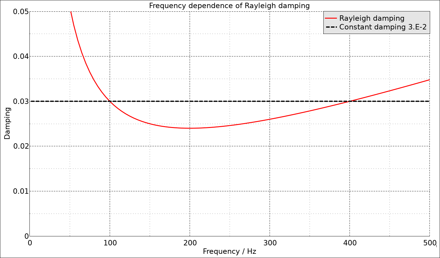
that Rayleigh damping is frequency dependent, with a damping ratio ξ
of:

The following plot shows the varying frequency-dependent damping ratio of Rayleigh damping. This also implies that the damping coefficients α and β depend on the unit system applied. Some optimization process may be required to find values of α and β that give a damping that is close enough to the desired damping ratio.
Stiffness Damping
The default implementation of stiffness damping
(*DAMPING_PART_STIFFNESS) is best suited for damping out high
frequency oscillations in explicit analyses. To obtain classical stiffness damping,
enter a negative damping value: COEF = -β. The stiffness
damping is introduced through a viscous term in the material routines. This requires
that IRATE < 1 on *CONTROL_IMPLICIT_DYNAMICS
for the stiffness damping to have effect.
For example, to introduce Rayleigh damping of approximately 3% in the frequency range 100 to 300 Hz on a global level, the following keyword template can be used:
*DAMPING_GLOBAL
0, 30.159
*SET_PART_LIST_GENERATE_TITLE
All parts for stiffness damping
338
1, 99999999
*DAMPING_PART_STIFFNESS_SET
338, -1.9099e-5
*CONTROL_IMPLICIT_DYNAMICS
1,
Approximately Frequency Independent Damping
Approximately frequency independent damping can be applied using the keyword
*DAMPING_FREQUENCY_RANGE_DEFORM. In this case, the fraction of
critical damping is given, and the frequency range for application,
𝐹low < 𝐹 <
𝐹high, is specified. The method is best suited
for small damping ratios (< 0.05) and frequency ranges such that 10 ≤
𝐹high/𝐹low
≤ 300.
The drawback with approximately frequency independent damping is that the dynamic stiffness of the model increases, leading to slight over-estimation of eigenfrequencies. This can be overcome by reducing the Young's modulus of the materials. For example, for 1% damping across a frequency range of 30 to 600 Hz, the average error across the frequency range is about 2%. It would therefore be appropriate to reduce the stiffness by (1.02)2, that is, by 4% in this case.
For example, to introduce approximately frequency independent damping of 3% in the frequency range 100 to 300 Hz on a global level, the following keyword template can be used:
*DAMPING_FREQUENCY_RANGE_DEFORM
3.E-2, 100., 300.,
Numerical Damping (Newmark Time Integrator)
The Newmark time integrator introduces numerical damping in the solution. The following figure compares the tip deflection for different nonlinear solutions of the example in Transient Loading of an L-beam.
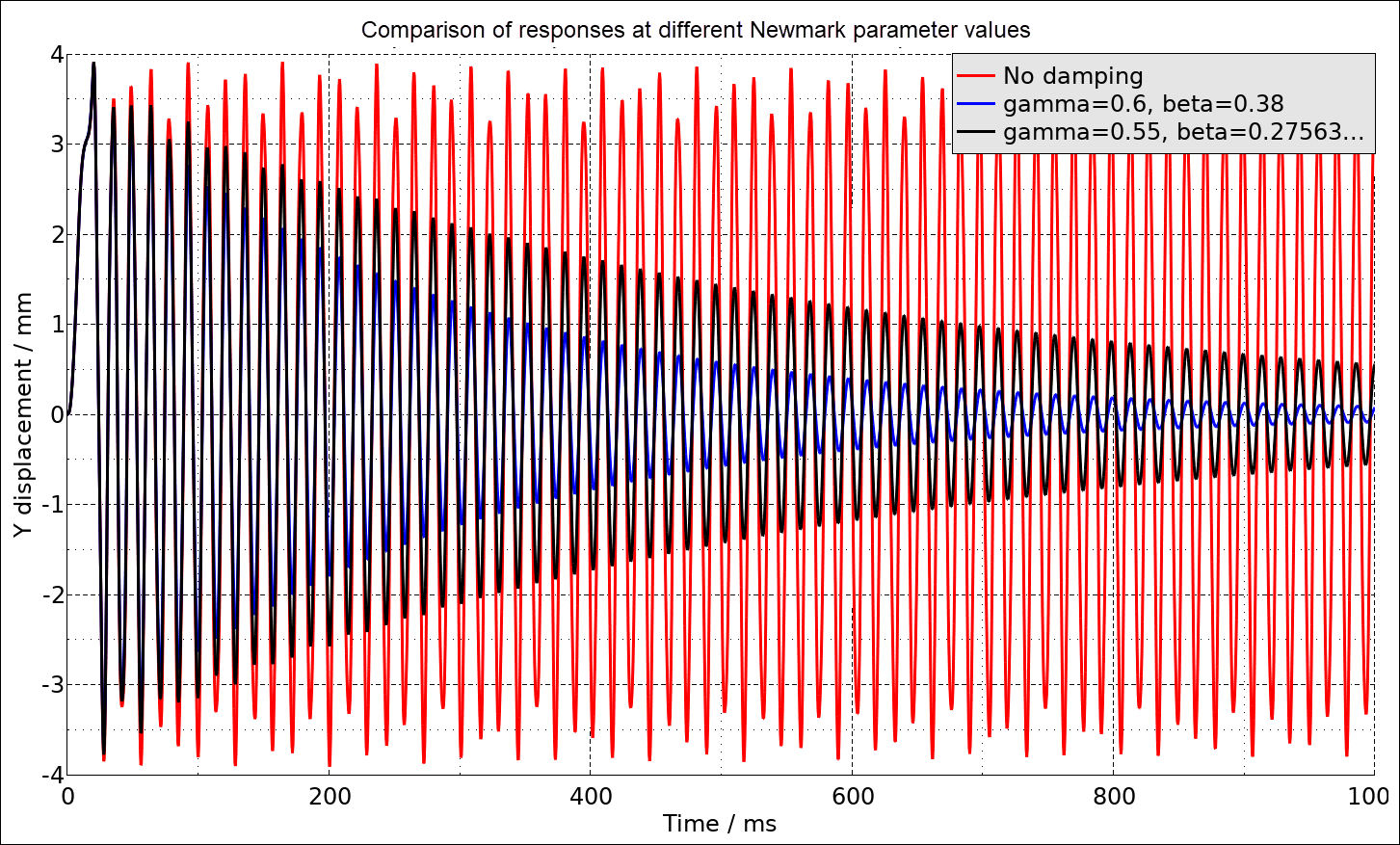
This artificial numerical damping is unphysical but may be beneficial in some situations because it can stabilize the solution and promote convergence. In addition to the settings of GAMMA and BETA, the numerical damping depends on the (lowest) natural frequency of the structure and the time step used in the numerical solution. See [32] for a discussion of numerical damping associated with implicit time integrators.
This example is very similar to the example in Transient Loading of an L-beam. Loads and boundary conditions remain the same, but a fully constrained, rigid transverse support (shown in green in the following figure) is added.
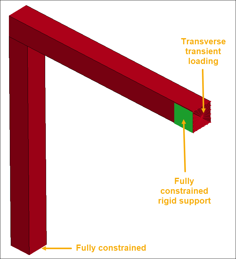
A contact condition is defined between the support and the beam using
*CONTACT_AUTOMATIC_SURFACE_TO_SURFACE_MORTAR. A
frequency-independent (for the range 50 - 300 Hz) damping of 3% of critical is
applied using *DAMPING_FREQUENCY_RANGE. Moderate numerical damping is
also applied by setting GAMMA = 0.55 and
BETA = 0.27563.
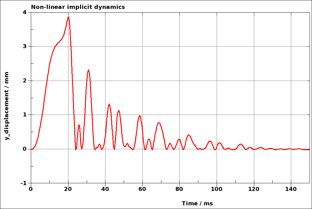
The transient displacement response of the loaded node is shown in the following figure. The response is quite chaotic at the beginning, but decays quickly due to the combined effect of the damping definitions.
The example keyword file is transient_nonlin001.key.