


This section examines the following trace mapping topics:
Import Trace Mapping
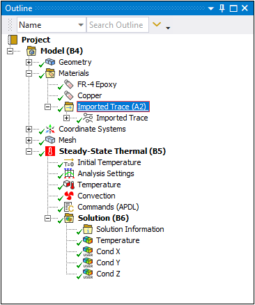
This step applies to the workflow for importing data from Workbench. In Mechanical, the application automatically inserts an Imported Trace folder and an Imported Trace object under the Material object.
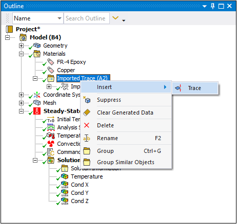
Using the context menu (right-click) option > enables you to insert additional Imported Trace objects into the tree as needed.
Specify External File
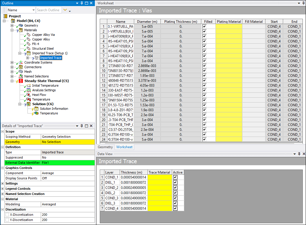
Once inserted, the Imported Trace: Vias Worksheet and the Data View window display. Once you specify the External Data Identifier property, source system data populates various application fields.
You can use the context (right-click) option on the Worksheet and Data View table to specify materials for the vias and imported traces.
Specify Properties and Settings
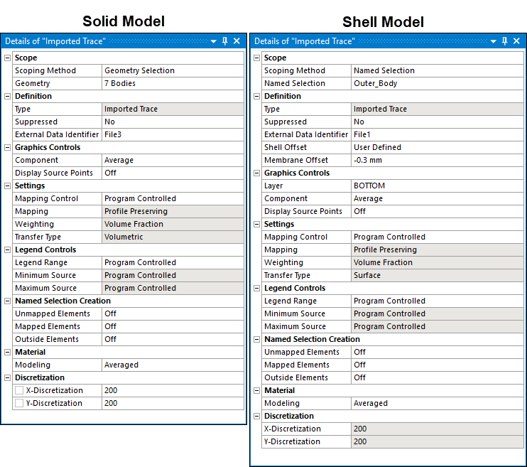
The Details view and the Data View for the Imported Trace object enable you to control the specification of the imported trace file in Mechanical.
The following options are available in the Details pane to control the Imported Trace specification.
Scope: The Geometry or the Named Selection properties, as specified by the Scoping Method property, support scoping to the bodies representing the layer geometry for the PCB or to elements contained on the layers of geometry.
You can model the geometry of a PCB as a shell or solid. When modeled as solid, you should model each layer as a separate body. When modeling shells, the application models all of the layers as a single shell geometry. Mechanical uses layered shell elements to model the layers of a PCB.
Note: Using the meshing Sweep Method Control, you can mesh a solid body with the Solid-Shell element (SOLSH190). This option is available from the Element Option property of the Sweep Method.
External Data Identifier: This property provides a drop-down list of available ECAD files from the list of files specified in the External Data system.
X-/Y-Discretization: Mechanical performs a two stage mapping to calculate metal fractions on the target mesh. First it computes a metal fraction distribution of the board from the source ECAD file to a regular grid, and then from the regular grid to the target mesh. The X-/Y-Discretization properties enable you to specify the size of the regular grid. The grid density count is x by default. Depending on the trace resolution and the computational costs desired, you can change the values for the rows and columns to receive optimum results. For accurate results, it is recommended that the X and Y discretization be specified such that the grid cell length be less than or equal to the minimum trace width. The Mechanical mesh size is recommended to be less than 4 times the grid cell length.
These fields are read-only when the ECAD File specified in External Data Identifier is of Icepak COND+INFO format and displays the discretization of the COND file.
Numerous additional properties are available in the Details. See the Data Transfer Mesh Mapping section for more information about these various properties
.
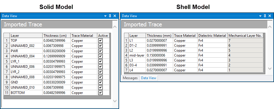
The Data View of the Imported Trace object enables you to see and/or control/override the following properties of the layers in the trace layout:
Layer: The name of the Layer.
Thickness: The thickness of the layers.
Trace Material: This property specifies the material for the metal traces on each layer. This material is created in the Engineering Data workspace for the Mechanical system.
Dielectric Material (shell geometry only): This property specifies the dielectric material for each layer.
This option is only available for traces scoped to shells. For imported traces scoped to solids, the base (dielectric) material is specified on the Material Assignment property of the selected bodies (under the Geometry object).
Active: This option enables you to activate or deactivate one or more layers. This option is not available for shell geometries. All layers are sent to the solver for traces imported on shells.
Mechanical Layer No.: Only available for traces scoped to shells. This read-only field displays the layer number by which this layer is identified. For example, if you want to post process results on the L1 layer show below, you will need to specify Layer 7 in the Details view of the result object.
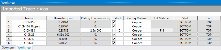
The Imported Trace: Vias Worksheet enables you to view and/or control and override the following properties of the vias in the trace layout.
| Column Heading | Column Description |
|---|---|
| Name | This field displays the name of the layer as defined in the source file. |
| Diameter | This read-only field displays the outer diameter value of the via. |
| Plating Thickness | This field displays the thickness of the interior wall of the via that is not filled. Only applicable when via is hollow (not filled). |
| Filled | Check and/or uncheck this fill to indicate whether the vias is filled or hollow. |
| Plating Material | When active, this field displays the metal material of the via. It provides a drop-down menu that enables you to specify different materials for the via. |
| Fill Material | This field provides a drop-down menu when the corresponding option is inactive, i.e. via is hollow (not filled). It enables you to specify a material for the hollow region of the via. You can assign Air (defined in Engineering Data) if the hollow region is empty. |
| Start/End | These read-only fields display the layer associated with where the via starts and ends. |
In addition to these basic controls, the Details view of the Imported Trace object provides additional properties that enable you to control/visualize the source data in Mechanical:
Display Source Points/Interior Points: These properties enable you to visualize the source points from the trace layout files. These settings can be used to verify the alignment of the source points with the target geometry. If misaligned, use the Rigid Transformation controls in the External Data system to align the source mesh with the target.
Mapping Control: This property controls mapping settings for the import. Options include (default) and . The option enables the application to determine the appropriate algorithm and settings based on the source and target mesh data, as well as the data type being transferred. See the Program Controlled Mapping topic in the Data Transfer Mesh Mapping section for additional information.
Interpolation: Options include (default) and . The option calculates effective conductivity by averaging the trace data in each element. Using the option, the application calculates the effective orthotropic conductivity for each element using the position and values of the trace data within each element.
- Directional Trace Mapping
This interpolation calculates orthotropic thermal conductivities for each element. The calculation is done by modeling the trace data in each element as a thermal resistance network. The examples illustrated below describe the calculated conductivity values based on the corresponding scenarios on the left. The dielectric in this example has a conductivity of 0.294 W/mK and the metal has a conductivity of 400 W/mK. Each element is 51% metal and 49% dielectric (Metal Fraction of 0.51).
Metal Fraction Kx (W/mK) Kx (W/mK) Kz (W/mK) 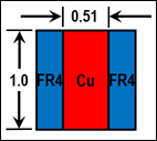
0.51 0.60 204.1 204.1 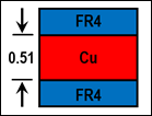
0.51 204.1 0.60 204.1 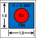
0.51 ~1 ~1 204.1 
Import Trace Layout Data
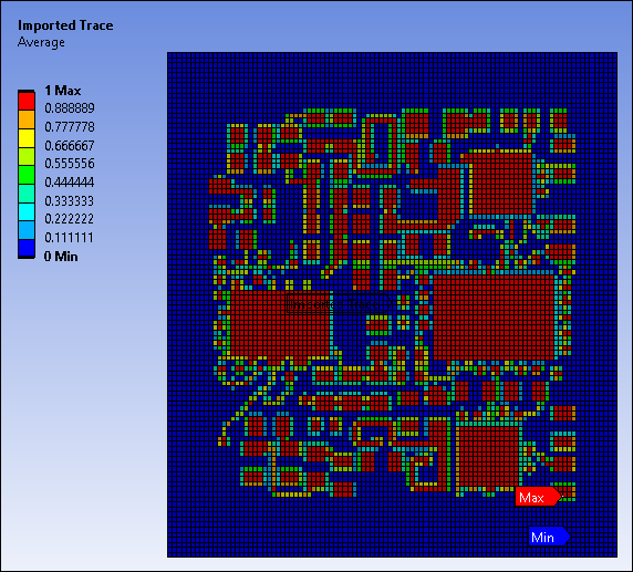
Once you have fully defined the object, right-click the Imported Trace object and select Import Trace to import the trace layout data onto the specified bodies. As illustrated below, the object displays the variable data, per element, of how much of the trace data is dielectric (metal) material. One (1) is 100% metal and zero (0) is 0% metal.
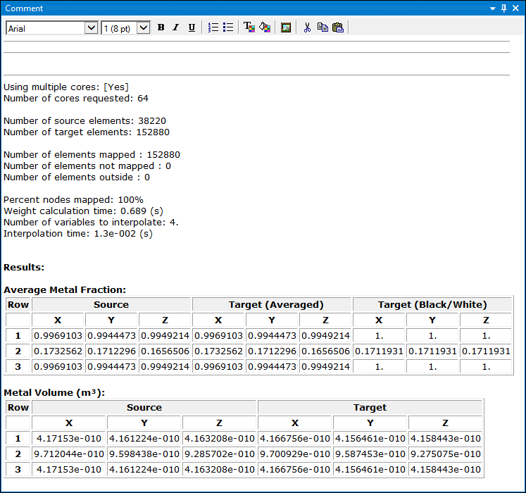
When you import trace layout data, the application generates the Imported Data Transfer Summary object. This object presents a summary, in the Comment pane, of the mapped source data as compared to target data. More specifically, it presents an average metal fraction for target elements, including both averaged modeling and black/white modeling. This enables you to validate your target metal fractions against the external application, such as Ansys Sherlock, you use to provide this metal fraction. However, unless the source data aligns perfectly to the target mesh, Ansys does not recommended that you compare the source and target average metal fractions.
In addition, the following properties in the Graphics category help to visualize the mapped data:
Component: X, Y, or Z component or the average of the imported metal fraction data.
Layer: Layer to display the data for (only applicable when scoped to shells)
Visualize Source Data
The source data can be visualized using the Validation object. To visualize the source data, use the context menu option > on the Imported Trace object to insert a Validation object in the tree. Once inserted, set the appropriate properties and use context menu option on the validation object. See Mapping Validation in the Ansys Mechanical User's Guide for details.
Apply Boundary Conditions
You can freely apply any supported boundary condition on solid bodies scoped to Imported Traces. Certain restrictions apply for boundary conditions on shell bodies scoped to Imported Traces. For example boundary conditions like Thermal Condition and Imported Body Temperature can only be applied to both the shell faces.
Solve the Analysis
The effects of Imported Trace data are included during the solution phase by computing the material properties of the materials assigned to the bodies based on the metal fraction. The Modeling property in the Material group controls how material properties are calculated based on computed metal fraction values. Two options are available:
: Assign trace material to regions with average metal fraction greater than or equal to 0.5, and dielectric to the rest.
: Calculate material properties based on calculated metal fraction. The supported material properties based on metal fraction are listed in the tables below:
- Thermal Analysis
The supported thermal material properties include:
Thermal Conductivity (Kx/Ky/Kz)
Specific Heat
- Structural Analysis
The supported structural material properties include:
Young's Modulus (Ex/Ey/Ez)
Poisson's Ratio (PRxy/PRyz/PRxz)
Coefficient of Thermal Expansion
Density
Note:Non-linear materials are not supported when is set to . If the application detects non-linear materials assigned either as trace or dielectric material when the material modeling is set to , then the Imported Trace object becomes invalid and the solution cannot proceed unless the conditions are made valid.
If any linear material properties other than the ones listed in the above table are present on either the trace or dielectric material, they are not sent to the solver.
When using LS-DYNA trace mapping, thermal analysis is not supported, and the coefficient of thermal expansion is not a supported material property.
Material Property Calculation for Temperature Dependent Material Properties
For temperature dependent material properties, averaging takes place over two stages. First the material properties are calculated at the union of all the temperatures, and then the average metal properties are calculated based on the above table for each temperature point. For example, the Metal material has property P specified at temperatures T1, T2 and T3, whereas the Dielectric material has property P specified at T2 and T4, then the material property is first calculated for both Metal and Dielectric materials at temperatures T1, T2, T3, and T4, and then the effective material properties are calculated at T1, T2, T3, and T4 using the table specified above.
- Offsets (Only applicable for shells)
When scoped to shells, the Shell Offset property allows user to specify the shell offset for the scoped bodies. Available options are and . The property allows you to specify the offset value.
Evaluate Results
Once the solution is complete, user can insert appropriate results and evaluate them. Since the effect of metal and dielectric within an element is captured through material property averaging, stress results may deviate from full fidelity analysis. However it provides a qualitative description of stress distribution. User may perform a subsequent Submodeling analysis to get accurate stress distribution.