


To transfer data across a dissimilar mesh interface, the nodes of one mesh must be mapped to the local coordinates of a node/element in the other mesh. This section describes the settings that are available in Mechanical when data is mapped across two different meshes.
You can add the exported mesh and loads as external data in the project schematic and couple a new Mechanical analysis system with this external data. The Mapping Settings described below are available within Mechanical for Thermal-Stress coupling with dissimilar mesh, Submodeling, when temperatures or displacements are transferred from Mechanical to Ansoft, or when the source data comes from an External Data system.
Mapping Settings
The Settings category provides the following properties.
- Mapping Control
By default, when Program Controlled is selected, the software will determine the appropriate algorithm and settings based on the source and target mesh data, as well as the data type being transferred. See Program Controlled Mapping topic below for additional information. You may choose to modify the advanced features by setting this to Manual.
- Mapping
This read-only property displays the mapping algorithms the application selects. Options include:
: Using this mapping option, the application simply takes the profile of the variable (for example, temperature) on one mesh, and matches or maps it to the other mesh as best as it can.
: Using this mapping option, the application makes sure that the profile is interpolated in such a way as to ensure that a total quantity passing across the interface is conserved, that is the same total passes out of one mesh and into the other. For example, a conservative interpolation of force ensures that the total force on one side of the boundary exactly matches the total force received by the other side of the boundary, even if the mesh resolution is poor. Conservative interpolation does not make sense for a variable such as temperature where there is no corresponding physical quantity to conserve.
Note: Conservative algorithms are only available for Imported Force loads. Conservative algorithms are not available for 2D to 3D data transfers. If conservative algorithms are not available, it is a read-only field displaying that a "Profile Preserving" algorithm is being used.
- Weighting
Choose which type of weighting should be performed. This option can be changed only if Mapping Control is set to Manual.
applies the source value directly on the nodes/elements identified by Node IDs/Element IDs in the External Data specification.
Note: This mapping only supports loads applied to nodes or elements. The following loads applied to element faces are not supported:
Pressure (on element faces)
Convection Coefficient
Heat Flux
Triangulation creates temporary elements from the n closest source nodes to find the closest points that will contribute portions of their data values. For 3D, 4-node tetrahedrons are created, and for 2D, 3-node triangles are created by iterating over all possible combinations of the source points (maximum number controlled by the Limit property), starting with the closest points. If the target point is found within the element, weights are calculated based on the target’s location inside the element.
Distance Based Average uses the distance from the target node to the specified number of closest source node(s) to calculate a weighting value.
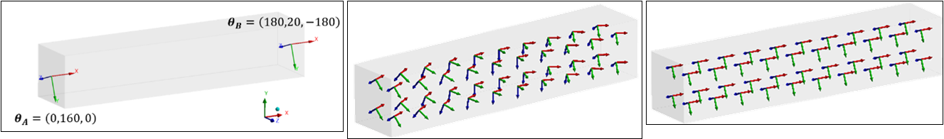
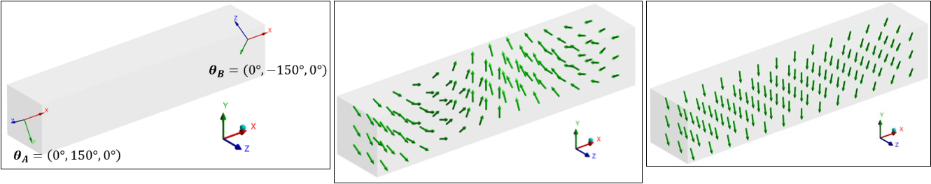
(Imported Element Orientations only) performs the interpolation in the quaternion space rather than directly on the Euler angles. Weighting values are calculated as in the case. All options available for the also apply to this Weighting type. This is the preferred approach for mapping orientations because:
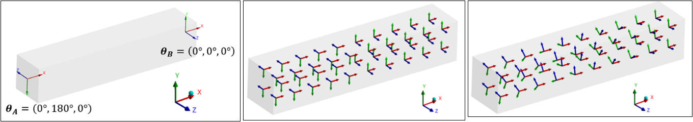
Several Euler angles parametrize the same orientation. Interpolating in the quaternion space enables the application to account for equivalence. See Figure 34. Quaternion interpolation provides the shortest path between two orientations as compared to interpolating the Euler angles directly, which can lead to counter-intuitive results. See Figure 35. Consider interpolating between same orientations A and B expressed with different (but equivalent) Euler angles (left). Euler angles interpolation (center) leads to counter-intuitive results. The quaternion interpolation (right) delivers the expected results (constant orientations over the part). Consider interpolating between the orientations A and B shown on the left. Quaternion interpolation (right) provides the shortest path between the two orientations, while Euler angles interpolation (center) takes the longest one. Weighting:
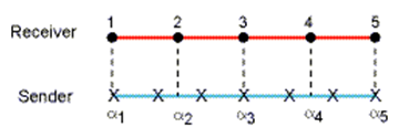
Shape Function: Two mapping methods are available for a load transfer: “Profile Preserving” and “Conservative”.
In a Profile Preserving mapping, each node on the target (receiver) side maps onto an element on the source (sender) side (α1). The transfer variable is then interpolated at α1. The transfer value is T1 = φ (α1). Thus, all nodes on the target side query the source side.
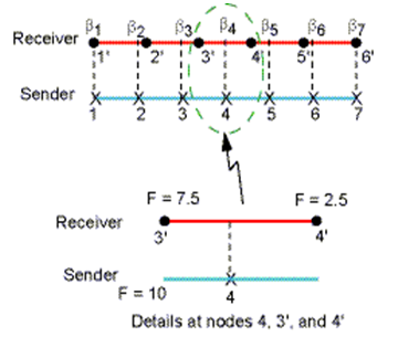
In a conservative mapping, each node X on the source (sender) maps onto an element on the target (receiver) side. Thus, the transfer variable on the source is split into two quantities that are added to the target nodes. As shown in the following figure, the force at node 4 splits into forces at nodes 3’ and 4’.
Thus profile preserving (conservative) version of Shape Function algorithm loops over the target (source) nodes and tries to locate a source (target) element that each target (source) node can be mapped to. Weights for each of the source nodes are then assigned based on the location of the target (source) node and the shape function of the element. For each target (source) node, the search efficiency can be improved by restricting the search to a subset of the source (target) elements. The search algorithm works by:
Distributing all source (target) elements into Cartesian boxes or buckets. The number of buckets is controlled by the Scale property.
Locating each of the target nodes in a box
Finding an element that each target (source) node can be mapped to by restricting the search with each target’s (source’s) box
Note:When there is a significant distance between target (source) node and the closest element, e.g. Shell-Solid submodeling, the node and the element may not be found in the same box. In order to improve mapping accuracy in such cases, the Pinball control may be used. See Pinball in the Advanced section for more details.
For conservative mapping, the value on a source node is distributed only on the nodes of the target element it is mapped to. Therefore, it is possible, especially if you are mapping from coarse to fine meshes, that some of the mapped target nodes get a zero value. This is because none of the adjacent elements are mapped to one or more source nodes.
For the Linux Platform, this mesh mapping option is limited to the use of only one processor core.
Kriging is a regression-based interpolation technique that assigns weights to surrounding source points according to their spatial covariance values. The algorithm combines the kriging model with a polynomial model to capture local and global deviations. The kriging model interpolates the source points based on their localized deviations, while the polynomial model globally approximates the source space. See Kriging in the DesignXplorer User's Guide for more information.
Note: By default, the Kriging technique uses an adaptive algorithm and ensures that the interpolated values do not exceed specific limits. The adaptive algorithm starts by using the higher-order Cross Quadratic polynomial to interpolate data. If the interpolated value of each target point is outside the extrapolation limit you specified, the algorithm re-interpolates data by reducing the polynomial order and the number of source points. Target nodes whose values are outside the limits when the lowest polynomial type is used are not assigned a value.
The Kriging algorithm, when used with the higher-order Cross Quadratic or Pure Quadratic polynomial, may fail to correctly interpolate data for a target point if multiple source points are spaced close to one another or if the target point is outside the region enclosed by the source points that are selected for interpolation. This may introduce gross errors in the estimation of the target value and manifests itself mostly when mapping data on surface or edge geometries. In such cases, you should change the Polynomial Type to Constant or Linear and, if necessary, reduce the number of source points to be included for the interpolation.
UV Mapping can be used to transfer data from one surface to another. Unlike other algorithms, UV mapping does not require the surfaces to be coincident. This allows for mapping between deformed and un-deformed geometries, as well as transfers between dissimilar geometry. Element data is required from both the source and the target mesh. If the source is an Mechanical APDL .cdb file containing volumetric element data, a nodal component must also be specified which will be used to define the surface from which the data transfer will occur.
Polyhedral Surface Creation and Conversion to UV
To map a mesh in UV space, the application first creates polyhedral surfaces from the given mesh data. If the source mesh is volumetric data, an associated node-based component must be selected such that the nodes consist of the surface area where the mapping takes place. Once the application creates the source and target surfaces, they are then ‘unfolded’ and converted into UV coordinates. The application defines the UV space as a parametric space where the axis data equals 0.0 to 1.0. Alignment points anchor the node locations to the corners of the 1x1 box.
Interpolation
Once the source and target data is converted to UV space, the target nodal UV locations are used to locate the source element that would contain the target node. The value for the target is then calculated based on the values provided from the source elements nodes.
Note: Available weighting options depend upon the data available from source and target and on the Mapping setting. Some of the weighting options may not be available for certain mesh data or Mapping settings. For example, when Mapping is set to Profile Preserving, Shape Function and UV are only available when the source provides element information. For Conservative Mapping, only Shape Function for Weighting and Surface for Transfer Type is available.
- Interpolation
Interpolation (Imported Trace only): This property species how the application calculates effective conductivity on a per element basis when you are performing an analysis that involves trace mapping of a circuit board. Options include (default) and . The option calculates effective conductivity by averaging the trace data in each element. Using the option, the application calculates the effective orthotropic conductivity for each element using the position and values of the trace data within each element.
- Transfer Type
Enables you to choose the dimension of the transfer (for 3D profile preserving transfers only). This option is available only for Triangulation, Shape Function, and for adaptive Kriging. For best results, use the Surface option when mapping data across surfaces and the Volumetric option when mapping data across volumes.
When used with Triangulation:
The Surface option tries to map each target point by searching triangles that are created from the set of closest source points. The target point will be projected onto the plane relative to the triangle surface. If the point is found inside the triangle, the weights are calculated based on the target’s projected location inside the triangle.
The Volumetric option tries to map each target point by searching tetrahedrons that are created from the set of closest source points.
When used with the Shape Function:
The Surface option uses the bucket surface search algorithm to locate a source element that each target node can be mapped to. This option supports only triangle and quadrilateral source elements; do not use it if your source elements are other shapes because the algorithm does not account for these shapes.
The Volumetric option uses the bucket volume search algorithm to locate a source element that each target node can be mapped to. This option supports triangle, quadrilateral, tetrahedron, hexahedron, and wedge source elements.
When used with adaptive Kriging, the Surface option uses fewer surrounding source points to interpolate data than the Volumetric option does.
- 2D Projection
Available only for 2D to 3D data transfers from an External Data system connected to Mechanical. The default option is Normal To Plane. You will be able to choose between the default as well as all application and user input coordinate systems.
Important: When you use a cylindrical coordinate system , the application projects the points on the mapped surface around the Z axis and into the ZX Plane on the positive X axis side.
Rigid Transformation
The properties of the Rigid Transformation category enable you to apply coordinate system transformations to the source points using the options of the Mesh Alignment property listed below.
Important:
For source data imported from an upstream External Data system, any transformation in Mechanical is added onto the Rigid Transformation performed in upstream External Data system.
Rigid Transformations are not supported when the Weighting property is set to .
The Mesh Alignment property includes two options:
- Use Origin and Euler Angles
You change the source point coordinate locations by specifying distance and rotational degree entries in the Origin and Theta properties. For example, an entry of 0.1 meters in the Origin X property would offset the X location of all the source points by 0.1 meters. In addition, it is important to note that rotational changes are made first and in the following order:
Theta ZX
Theta YZ
Theta XY
Once complete, translational changes are made.
- Use Coordinate Systems
When you select this option, the Source Coordinate System and the Target Coordinate System properties display. Each property provides a drop-down list of available coordinate systems to select from. Based on your selections, the transformations are calculated so that the Source Coordinate System automatically aligns with the Target Coordinate System. For example, when the source mesh is defined in the XY plane, whereas the target geometry is defined in a plane obtained by applying the Euler rotations RXY, RYZ and RZX to the XY plane. Then choosing Global Coordinate System as Source Coordinate System and the coordinate system created by applying the transformations RXY, RYZ and RZX to the Global Coordinate System as the Target Coordinate Systems, the source mesh is transformed such that it is aligned with the target geometry. This option is useful if the source points are defined with respect to a coordinate system that is not aligned with the target geometry system.
Note: When your upstream system is an External Data system, the default option for both properties is . This internal coordinate system is not visible in the Outline. It represents the coordinate system that transformed the source points in the External Data system. If there are no Rigid Transformations defined in the upstream External Data system, the is the same as the .
Note: For an Imported Load or Imported Thickness object, set the Display Source Points property to to display the alignment of the source and target points.
Graphics Controls
The Graphics Controls category provides the following properties.
Display Source Points: Toggle display of source point data. This can be helpful in visualizing where the source point data is in reference to the target mesh.
Display Source Point Ids: Toggle display of source point identifiers. This can be helpful in conjunction with validation objects when trying to identify nodes with undefined values. Note that if a column is not defined with the Node ID Data Type, the source point ids will correspond to the row from which they come in the file. For formatted and delimited files, ids will start after skipped lines.
Display Interior Points: Available when Display Source Points or Display Source Point Ids is set to On. Toggle allowing source point data to be displayed through the model so that interior points can be seen.
Display Projection Plane: Toggle display of project plane (available only for 2D to 3D mapping).
Legend Controls
The Legend Controls category provides the following properties.
Legend Range: Program Controlled (default) or Manual control of the legend minimum and maximum values. When Program Controlled is selected, the target data's minimum and maximum values will be used in the legend. When Manual is selected, control of the Maximum and Minimum values can input and the graphics will be drawn based on these values.
Minimum: When Legend Range is set to Manual, this option is available for inputting the minimum legend value.
Maximum: When Legend Range is set to Manual, this option is available for inputting the maximum legend value.
Source Minimum: Read only field providing the source data minimum value.
Source Maximum: Read only field providing the source data maximum value.
Named Selection Creation
The Named Selections category provides the following properties.
Unmapped Nodes: Activating this property creates a named selection containing all of the points that cannot be mapped. The default setting is Off.
In addition, when you activate this property, an associated Name property displays. This property displays the name of the Named Selection. You can edit this field. By default, the application assigns name "Unmapped Nodes."
Mapped Nodes: Activating this property creates a named selection that contains all mapped points. The default setting is .
In addition, when you activate this property, an associated Name property displays. This property displays the name of the Named Selection. You can edit this field. By default, the application assigns name "Mapped Nodes."
Outside Nodes: Activating this property create a named selection containing all the points that cannot be found within tetrahedrons/triangles when Triangulation is used. The default setting is .
In addition, when you activate this property, an associated Name property displays. This property displays the name of the Named Selection. You can edit this field. By default, the application assigns name "Outside Nodes."
These settings are only available for profile preserving mapping.
Advanced
The application filters the properties of the Advanced category based on the settings made in the Mapping Control and Weighting properties in the Mapping Settings category. Properties include:
Pinball: The Pinball property enables you to specify a region of interest around a target point. Only the source points/elements inside the pinball region are considered for mapping and any point/element outside of the pinball will not be used. Specific behavior of the Pinball control is dependent on the Weighting type selected as discussed below:
When used with Triangulation or Distance Based Average, a bounding box is created around the target point based on the value of the pinball to find the closest source points. Any point outside of the bounding box will not be used. By default, the Program Controlled value is 0.0, which calculates the distance based on .05% of the source region's bounding box size. The bounding box will automatically resize if the mapping is unable to find the minimum number of points required to calculate weighting factors. (Note that resizing occurs only for Program Controlled.)
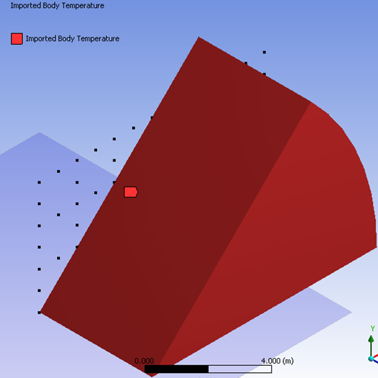
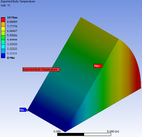
Note: In certain cases when Pinball is set to Program Controlled, the process of searching for source nodes around a target node can take a long time. In the image below, the target nodes are located on the red face. The target nodes (A) closest to the vertical body will quickly find nodes in the +Y axis direction. Target nodes (B) further down the X axis will take longer to find.
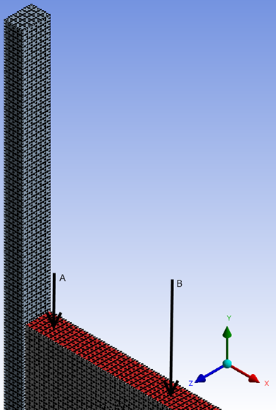
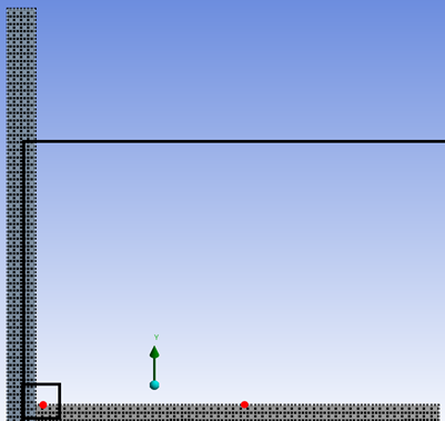
As an example, consider the case shown in the image below. The two red dots indicate target nodes in regions A and B. For each target node, the triangulation algorithm will begin its search for source nodes within the perimeter of a psuedo cube (bounding box) centered at its location. For the first pass, the edge length of the cube is set to be 0.05% of the maximum bounding box length of the source region. The algorithm looks to find ‘n’ source points (set by the limits property) in the positive and negative X, Y, and Z axes of the cube. If ‘n’ source points cannot be found in any of the six directions (±X, ±Y, and ±Z), the size of the search region is doubled and the process repeated. The search process continues until the required number of source points are found in all directions or until the search region extends beyond the limits of the source bounding box.
During the first pass, for the target node in region A, the algorithm is able to find the required number of source nodes. However, for the target node in region B, sufficient nodes cannot be found in the +Y direction and the size of the search area is increased. As illustrated in the figure below, for the target node in region B, the algorithm runs through several iterations before it is able to find the required number of source nodes. This results in an increase in time as well as the possible inclusion of source nodes that are significantly further away from the target node.
Please note that for each target node the pinball is reset to its initial size (0.05% of the maximum bounding box length) before the search begins.
For such cases it is recommended that you specify a pinball value so that the search box can be controlled to only find nodes within a certain region. This allows for triangulation to quickly search for source nodes, as well as to ignore source nodes that are sufficiently far away from the target node.

When used with Shape Function, the Pinball control can be used to:
Exclude from mapping to elements far away from the target point. When Transfer Type is Surface, the target point is projected onto the source elements to find the matching element. Due to projection, the gap (the distance between target point and its projection on the matching element) between the target point and the matching element may be large. Such elements are excluded from mapping if the gap is larger than the Pinball Value specified.
Expand the search region to find matching elements. Shape function algorithm works by distributing the source elements into regions called buckets, and then for each target point, finding the appropriate bucket and searching for the matching element in the bucket. When there is a significant distance between a target node and the closest element, e.g. Shell-Solid submodeling, the node and the element may not be found in the same bucket. In order to improve mapping accuracy in such cases, the Pinball control may be used to include additional buckets for mapping. When a Pinball Value greater that 0 is specified, then a bounding region is created around the target node using the Pinball Value and all the buckets associated with the region are used to find the appropriate element. To improve the mapping efficiency, the search is restricted only to the elements within the bounding region.
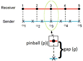
α3 is excluded when pinball (p) < gap (g), and included when pinball (p) ≥gap (g).
The Pinball option is not available when Weighting is set to Kriging.
Limit: Number of nearby points considered for interpolation. Defaults to 20. Lower values will reduce processing time, however, some distorted or irregular meshes will require a higher Limit value to successfully encounter nodes for triangulation.
When Weighting is set to Kriging, the minimum value that can be used is based on the selected Polynomial type.
Weighting Minimum Limit Maximum Limit Triangulation 5 20 Kriging (Constant) 3 (3D), 2 (2D) Number of source points Kriging (Linear) 4 (3D), 3 (2D) Number of source points Kriging (Pure Quadratic) 7 (3D), 5 (2D) Number of source points Kriging (Cross Quadratic) 10 (3D), 6 (2D) Number of source points Outside Option: Enables you to ignore or choose a different weighting algorithm for target points that cannot be found within the source mesh/points. Different options are available, based on the Weighting option chosen:
When used with Triangulation. For target points that cannot be found within tetrahedrons/triangles created for Triangulation.
Distance Based Average: The mapping will use a weighted average based on distances to the closest Number of Points. Distance Based Average is the default option.
Ignore: Target points will be ignored and no value will be applied.
Projection: Triangles will be created from the closest Number of Points and the target point will be projected onto the plane relative to the triangle surface. If the point is found inside the triangle, the weights are calculated based on the target’s projected location inside the triangle. This option is available only for 3D transfers when the Transfer Type is set to Volumetric.
When used with Shape Function. For target points that cannot be found within source elements.
Nearest Node: The mapping will use the data from the nearest source node.
Ignore: Target points will be ignored and no value will be applied.
Note:For the Conservative Shape Function algorithm, the source mesh is mapped onto the target mesh (as opposed to profile preserving version, which maps target mesh onto source), and outside options control the contribution from source nodes which fall outside the target mesh.
Nearest Node is the default option for the Profile Preserving Shape Function algorithm, while the Ignore option is the default for the conservative algorithm.
Number of Points: When Weighting is set to Distance Based Average, or when Outside Option is set to Distance Based Average or Projection, this option is available to specify how many closest source points should be used when calculating weights. Valid range is from 1 to 8 for Distance Based Average and 3 to 20 for Projection. Defaults to 3.
Outside Distance Checking: When Weighting is set to Triangulation and Outside Option is set to Distance Based Average or Projection, this option enables you to specify a Maximum Distance cutoff beyond which source points will be ignored. Defaults to Off. The maximum number of source points is limited to the value specified by the Number of Points setting.
If the Outside Option is set to Distance Based Average, only source points that lie on or within a sphere (centered at the targets location and radius defined by the Maximum Distance value) will provide contributions.
If the Outside Option is set to Projection, the algorithm only uses triangles with centroids that lie on or inside a sphere (centered at the targets location and radius defined by the Maximum Distance value).
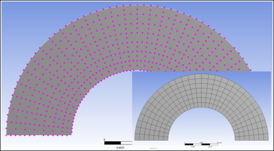
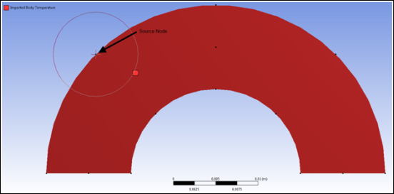
In Figure 5: Outside Nodes (Pink) with Mesh Overlay, all the pink nodes on the surface are found “Outside” the source points and will use the Outside Distance Checking based on the Maximum Distance specified.
In Figure 6: Maximum Distance set to 0.005 (m), the circle is at the mouse location with radius set to 0.005 (m). Nodes within this radius will be mapped. The source nodes are drawn as black dots and come from an extremely coarse mesh.
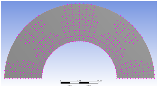
In Figure 7: Mapped Nodes, the “Outside” nodes get mapped because they are located within the Maximum Distance.
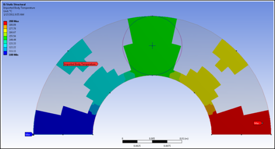
The result of the import is shown in Figure 8: Imported Data using Maximum Distance for Outside Nodes. Transparent areas show target nodes that do not get mapped because there are no source nodes within the Maximum Distance.
When Weighting is set to Kriging, this option allows you to ignore target points that lie outside the source bounding box. Defaults to Off. When this option is set to On, the Bounding Box Tolerance property enables you to include target points that lie outside the source bounding box by specifying a tolerance value. The algorithm adds this tolerance value to the source bounding box when it checks to see if a target point should be ignored or not.
Scale: When weighting is set to Shape Function, the scaling factor (%) determines the number of buckets used to distribute the source elements. Defaults to 50% (2 buckets).
Edge Tolerance: Dimensionless mapping tolerance (default = 0.05).
Shape Function for Surface/Edge topology.
Correlation Function: When weighting is set to Kriging, this property enables you to change the mathematical function that is used to model the spatial correlation between the sample points. Defaults to Gaussian.
Polynomial: When weighting is set to Kriging, this property enables you to change the mathematical function that is used to globally approximate the sample. Defaults to Adaptive.
Extrapolation Tolerance: You can use this option with adaptive Kriging to ensure that the interpolated value for each target point lies within specific limits. The tolerance is applied to the source range (based on the source points used for each target point) to determine if the interpolated value is satisfactory or if the data needs to be re-interpolated by reducing the polynomial order and the number of source points. For example, consider a target point having source values between 99 and 100. The default tolerance value of 10% will ensure that the mapped value is between 98.9 and 100.1. Target points whose values are outside the limits when the lowest polynomial type is used are not assigned a value.
: This option is available when the Weighting property is set to . When selected, the interpolation calculation treats orientations that have been flipped as equivalent. That is, given an element orientation identified by the axes (X,Y,Z), the algorithm treats as equivalent the orientations (X,Y,Z), (-X, -Y, Z), (X, -Y, -Z), and (-X, Y, -Z). See Figure 45.
Consider interpolating between the orientations A and B shown on the left. Note that A can be obtained by flipping the Z axis in the reference coordinate system. Mapped orientations obtained with and without Orientation Realignment are shown in the center and right, respectively.
Advanced Shell-Solid
Advanced shell-solid settings are filtered based on the Mapping Control and Weighting type selected in Mapping Settings. They are only available for Shell-Solid submodeling. In the case of imported cut boundary conditions, Shape Function is the only available Weighting type.
Pinball Factor: This value is used to calculate the Pinball Value for shell-solid submodeling. The Pinball Value is calculated by scaling the maximum shell thickness with the Pinball Factor.
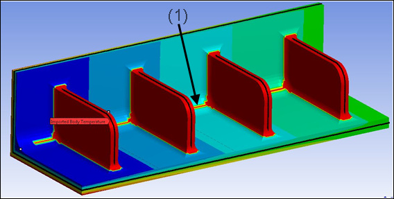
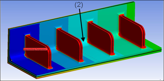
As shown in Figure 10: Shell-Solid Submodeling with Pinball Factor = 1.0 and Figure 11: Shell-Solid Submodeling with Pinball Factor = 1.2, the gap between the nodes in the filleted region is greater than the maximum shell thickness for the model. Hence using a Pinball Factor equal to 1 results in nodes in the fillet not finding appropriate matching elements.(1) When Pinball Factor of 1.2 is used, then additional buckets are included in the search resulting in better mapping results.(2)
Note: Increasing the Pinball Factor increases the number of buckets searched to find the matching element hence, may decrease the efficiency of the mapping. An appropriate value should be chosen so that the resulting bounding region includes the matching element but not too big so as to negatively affect the efficiency of the search.
Shell Thickness Factor: For shell models with variable thickness, the gap between the target node, and matching element may be large. Shell Thickness Factor is used to exclude any matching element which has a gap greater than Thickness* Shell Thickness Factor. Thickness is the average element thickness of the matching element.
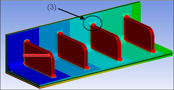
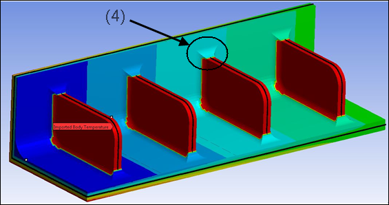
Note: Increasing the Shell Thickness Factor to allow submodel nodes to be “found” can produce poor submodel results as shown in Figure 12: Shell-Solid Submodeling with Shell Thickness Factor = 0.6 and Figure 13: Shell-Solid Submodeling with Shell Thickness Factor = 1.2. where large Shell Thickness Factor causes the target nodes on the web region to be matched with the base (3), whereas the target nodes are more appropriately matched for a smaller Shell Thickness Factor (4).
UV Source Controls/UV Target Controls
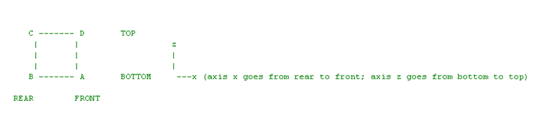
Alignment: Program Controlled (default) or Manual control of selecting the four alignment points needed for UV Mapping. The process of UV mapping involves aligning both the source and target nodal data from XYZ coordinates into the equivalent UV space. To do this, the mapper needs to have access to four alignment locations as reference points for unfolding and flattening the nodal information. These four locations are referred to as “Front Bottom”, “Rear Bottom”, “Rear Top”, and “Front Top”. When the Program Controlled alignment option is selected, the associated coordinate systems ZX plane is used in relation to the associated mesh nodal locations.
Coordinate System: Available when Alignment is set to Program Controlled. One of the available coordinate systems must be selected as a reference point for Program Controlled alignment. The mesh nodal data is transformed related to the ZX plane of the selected coordinate system. A mean Z value is determined so that the nodes can be split into 2 groups, an upper and lower section. The nodes in each section are then sorted based on their X position. If there are nodes at the same X position, these points are then sorted based on their Z location. For the “Rear Bottom” and “Front Bottom” points, the minimum sorted Z point will be used, and for the “Rear Top” and “Front Top”, the maximum Z point will be used.
Nodes: Available when Alignment is set to Manual for UV Source Controls. The user must list the 4 node locations in the text entry separated by commas. The order must be input as Front Bottom, Rear Bottom, Rear Top, Front Top.
Target Front-Bottom, Target Rear-Bottom, Target Front-Top, Target Front-Top: Available when Alignment is set to Manual for UV Target Controls. The user must select geometric vertices for each alignment point.
Program Controlled Mapping
Refer to the following table for the appropriate settings for when you set the Mapping Control property to in order to determine which type of mapping algorithm to use. The application determines default settings based on the properties described above.
When Mapping is Profile Preserving:
| Source mesh can provide: | Target mesh can provide: | Weighting that will be used: |
|---|---|---|
| Node IDs Only | Nodes | Uses to assign values to target nodes. |
| Element IDs Only | Elements | Uses to assign values to target elements. |
| Nodes Only | Nodes Only | Uses Triangulation to calculate mapping data. |
| Nodes and Elements | Nodes Only | Uses Shape Function to calculate mapping data. |
When Mapping is Conservative
| Source mesh can provide: | Target mesh can provide: | Weighting that will be used: |
|---|---|---|
| Nodes Only | Nodes and Elements | Uses Shape Function to calculate mapping data. |
Manual Mapping
When manual mode is selected, you will be able to control advanced settings for the mapper. Based on the mapping chosen (conservative or profile preserving) and mesh data provided from the source and target, you will be able to choose the type of weighting algorithm.
For Profile Preserving Mapping:
If the source mesh contains only points, you will be able to select from the following:
Direct Assignment (requires source Node or Element IDs)
Triangulation
Distance Based Average
Kriging
If the source mesh also contains element data, you will have the items listed above as well as:
Shape Function
For Conservative Mapping:
If the source mesh contains only points, you will be able to select from the following:
Shape Function
Element shapes supported during mapping when Shape Function is selected:
| Element Shape | Supported |
|---|---|
| 3 Node Triangle | X (2D) (3D) |
| 6 Node Triangle | X (2D) (3D) |
| 4 Node Quadrilateral | X (2D) (3D) |
| 8 Node Quadrilateral | X (2D) (3D) |
| 4 Node Tetrahedron | X (3D) |
| 10 Node Tetrahedron | X (3D) |
| 8 Node Hexahedron | X (3D) |
| 20 Node Hexahedron | X (3D) |
| 6 Node Wedge | X (3D) |
| 15 Node Wedge | X (3D) |
2D to 3D Mapping
Mapping point data from 2D to 3D analyses is possible using the External Data system connected to a downstream Mechanical system. This mapping is performed by collapsing the 3D mesh data into a 2D plane and calculating target point weighting factors from the source point data.
2D results in the XY Plane:
You will be able to select the 2D project plane to use based on the available coordinate systems as well as an option to select normal to the 2D source point data (Normal To Plane). Using the Graphics Controls described above, you will be able to turn on and off visualization of the source point data and the 2D projection plane.
Source point and 2D projection plane displayed:
When selecting Cartesian coordinate systems, the projection will be done on the XY Plane. If the coordinate system is cylindrical, the projection will be rotated about the Z axis into the ZX Plane. Normal To Plane will project the target points into the source point plane.
3D mapped data using cylindrical coordinate system projection:
3D mapped data using Normal To Plane:
Note: Conservative mapping is not available for 2D to 3D transfers.
Notes
When mapping point cloud data, the mapping utility does not know where body boundaries are. If you have a model with contact between two bodies, the mapping may pick up points from both bodies causing undesired results.