


If your analysis has load data defined from External Data, an Imported Load (External) folder is added under the Environment folder. Unless otherwise specified, the following steps apply to loads imported from a text (.txt) file.
To add an imported load, select the Imported Load folder and select a desired load from the Imported Loads drop-down menu on the Environment Context tab or right-click the Imported Load folder and select the appropriate load from the context menu.
Select appropriate geometry or mesh entity.
In a 3D structural analysis, if the Imported Body Temperature load is scoped to one or more surface bodies, the Shell Face option in the Details pane enables you to apply the temperatures to Both faces, to the Top face(s) only, or to the Bottom face(s) only. See Imported Body Temperature for additional information.
When mapping data to surface bodies, you can control the effective offset and thickness value at each target node, and consequently the location used during mapping, by using the Shell Thickness Factor property. By default, the thickness value at each target node is ignored when data is mapped.
You can choose to enter a positive or negative value for the Shell Thickness Factor. This value is multiplied by each target node’s physical thickness and is used along with the node’s offset to determine the top and bottom location of each target node. A positive value for the Shell Thickness Factor uses the top location of each node during mapping, while a negative value uses the bottom location of each node. For example:
A value of 0.0 means that the physical thickness and offset of the surface body nodes will be ignored; all target nodes are mapped at default surface body locations.
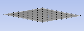
A value of 1.0 means that the thickness used for a target node will be equal to the physical thickness value specified for that node. The top location of the node will be used during the mapping process. The image below depicts a change to the position of the nodes, but this is not a reflection of what you will see in the application.
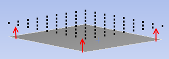
A value of -2.0 means that the thickness used for a target node will be equal to twice the physical thickness value specified for that node. The bottom location of the node will be used during the mapping process. The image below depicts a change to the position of the nodes, but this is not a reflection of what you will see in the application.
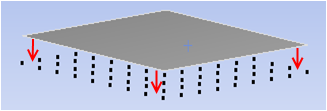
The view will look similar to the following for a value of –1.0. The colored dots represent the location and corresponding values of the source nodes. In this case, each target node will be projected using its physical thickness value to its bottom location and then mapped.
Select appropriate options in the Details pane. You can modify the Settings category properties to achieve the desired mapping accuracy. And, mapping can be validated by using mapping Validation for an object.
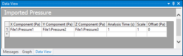
For pressure loads, you can apply the load in the direction normal to the face or by specifying a direction. Setting Define By to Components enables you to define the direction by specifying the x, y, and z magnitude components of the load. The z component is not applicable for 2-D analyses. For pressure loads in Harmonic Response, you can apply both real and imaginary components of the loads.
In a 3D analysis, if the Triangulation mapping algorithm is used, the Transfer Type mapping option defaults to Surface when an Imported Temperature or Imported Body Temperature load scoping is only on shell bodies. If the scoping is on shell bodies and other geometry types, the Transfer Type mapping option will default to Volumetric. In such cases, to obtain a more accurate mapping, you should create a separate imported load for geometry selections on shell bodies, and use the Surface option for Transfer Type. See Transfer Type under Mapping Settings for additional information.
For Imported Pressure loads, you can apply the load onto centroids or corner nodes using the Applied to property in the Details view. See Imported Pressure for additional information.
For imported force loads, both conservative and profile preserving algorithms are available using the Mapping property. See Imported Force and Mapping Settings for additional information.
For each load step, if an Imported Displacement and other support/displacement constraints are applied on common geometry selections, you can choose to override the specified constraints by using the Override Constraints option in the details of the Imported Displacement object. By default, the specified constraints are respected and imported displacements are applied only to the free degrees of freedom of a node.
For Vector[1]and Tensor[2]loads, the Coordinate System property can be used to associate the component identifiers, defined in the worksheet, to a particular coordinate system. This option is useful when the source data is defined, or needs to be defined, with respect to a coordinate system that is not aligned with the Global coordinate system. If a cylindrical coordinate system is chosen, the data is interpreted to be in the radial, tangential, and axial directions. By default, the Source coordinate system is used.
Note: The option of the Coordinate System property is an internal coordinate system that is not visible in the Outline. This coordinate system represents source points transformed first by Rigid Transformation process in the upstream External Data system and then by the Rigid Transformation process in the Mechanical application. If there are no rigid transformations from the upstream External Data system or in Mechanical, then the is the same as the .
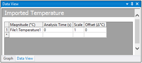
Under Data View, select the desired data Identifier for the imported load. The data identifier (File Identifier: Data Identifier) strings are specified in External Data. You can also change the Analysis Time/Frequency and specify Scale and Offset values for the imported loads.
For Vector[1] and Tensor[2] loads, if the Define By property is set to Components you should select data identifiers that represent the x/radial, y/tangential, and z/axial magnitude components of the load. For Vector[1] and Tensor[2], the components are applied in the Coordinate System specified in the Details view. The z component is not applicable for 2-D analyses. For Imported Displacement load, you can choose to keep a component free, or fixed (displacement = 0.0) by selecting the Free or Fixed option from the list of data identifiers. For all other loads, you can choose to ignore a component if you do not have data for that direction by selecting the Ignore identifier from the drop-down list.
For Imported Body Force Density/Imported Pressure/Imported Velocity in Harmonic Response analyses, you should select data identifiers for both real and imaginary components. You can also specify Scale and Offset for both real and imaginary components.
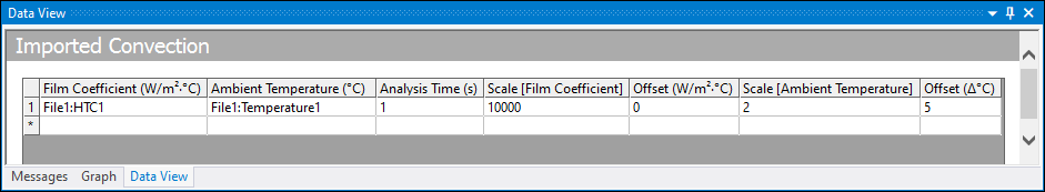
For Imported Convections, you should select data identifiers for film coefficient and ambient temperature. You can also specify Scale and Offset values for both film coefficient and ambient temperature.
Right-click in the Data View and select Add row to specify additional data for a different analysis time/frequency.
Change any of the columns in the Data View tab as needed:
Magnitude/Film Coefficient/Ambient Temperature
Select the appropriate data identifier that represents the load values to be applied from the drop-down list.
X Component
Select the appropriate data identifier that represents the x component of the load values to be applied from the drop-down list.
Y Component
Select the appropriate data identifier that represents the y component of the load values to be applied from the drop-down list.
Z Component
Select the appropriate data identifier that represents the z component of the load values to be applied from the drop-down list.
Note: If you do not have data for a direction you can choose to ignore that component by selecting Ignore from the appropriate drop-down box. Select the Fixed option from the drop-down list to make the component constant with a value of zero or the Free option for the component to be without any constraints.
If multiple files have been used in External Data, the data identifiers for component-based vector or convection loads must come from the same file(s) that have a primary file association. For example, you can select File1:PressureX, File1:PressureY, and File1:PressureZ, but you cannot select File1:PressureX, File2:PressureY, File3.PressureZ (assuming that File1, File2, and File3 do not have a primary file association).
XX, YY, ZZ, XY, YZ, and ZXComponent
Select the appropriate data identifiers to represent the components of the symmetric tensor to be applied from the drop-down list.
Analysis Time/Frequency
Choose the analysis time at which the load will be applied.
Scale
The amount by which the imported load values are scaled before applying them.
Offset
An offset that is added to the imported load values before applying them.
In the Outline, right-click the Imported Load, and then click Import Load to import the load.
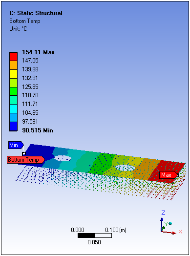
When the load has been imported successfully, a contour or vector plot will be displayed in the Geometry window.
For Vector[1] loads, contours plots of the magnitude (Total) or X/Y/Z component can be viewed by changing the Data option in the details pane. Defaults to a vector plot (All).
For Tensor2 loads, contours plots of the Equivalent (von-Mises) or XX, YY, ZZ, XY, YZ and ZX components can be viewed by changing the Data option in the details pane. Defaults to a Vector Principal plot.
For Imported Convections loads, contours plots of film coefficient or ambient temperature can be viewed by changing the Data option in the details pane.
For complex load types, such as Pressure/Velocity in Harmonic Response, the real/imaginary component of the data can be viewed by changing the Complex Data Component option in the details pane.
Note:Many imported loads as well as Element Orientations support Vector Display options.
The range of data displayed in the graphics window can be controlled using the Legend controls options. See Imported Boundary Conditions for additional information.
If multiple rows are defined in the Data View, imported values at different time steps can be displayed by changing the Active Row option in the details pane.
To activate or deactivate the load at a step, highlight the specific step in the Graph or Tabular Data window, and choose Activate/Deactivateat this step! See Activating and Deactivating Loads for additional rules when multiple load objects of the same type exist on common geometry selections.
Important:
For Vector[1] and Tensor[2] loads, when the Define By property is set to Components:
Any transformations specified in External Data and/or in Mechanical, are applied to the mapped data if the Coordinate System property is set to . If another Coordinate System is specified, then the components are applied in that Coordinate System.
Rotations produced by a cylindrical projection coordinate system, for 2D to 3D mapping, are also applied to the mapped data. Rotations resulting from analytical transformations specified in External Data, do not get applied to the mapped data.
For Imported Displacements, selecting the Free identifier for a source component will result in the corresponding target component being left unconstrained and free to deform in that direction, whereas Fixed identifier results in a value of zero being applied. For other load types, a value of zero is applied on selecting the Ignore component.