


A Hydrostatic Pressure load simulates pressure that occurs due to fluid weight.
This page includes the following sections:
Analysis Types
Hydrostatic Pressure is available for the following analysis types:
Dimensional Types
The supported dimensional types for the Hydrostatic Pressure boundary condition include:
3D Simulation
2D Simulation
Geometry Types
The supported geometry types for Hydrostatic Pressure include:
Solid
Surface/Shell
Topology Selection Options
The supported topology selection options for the Hydrostatic Pressure boundary condition include:
Face: Supported for 3D only.
Edge: Supported for 2D only.
Define By Options
The supported Define By options for the Hydrostatic Pressure boundary condition include:
(default)
Note: The vector load definition displays in the Annotation legend with the label Components. The Magnitude and Direction entries, in any combination or sequence, define these displayed values. These are the values sent to the solver.
When using the Mechanical APDL solver, for all of the above Define By property options, the Hydrostatic Pressure boundary condition also displays the Applied By property. This property has two options: (default) and .
The option applies pressure using the surface effect elements created on the top of the scoped geometry. The option applies pressure directly onto the faces of solid or shell elements in 3D analyses. In 2D analyses, the option applies pressure directly onto the edges of plane elements.
Note:
If you scope two Hydrostatic Pressure objects to the same geometry, and specify the loads in the same direction, using the option, the pressures do not produce a cumulative loading effect. The Hydrostatic Pressure object that you specified last takes priority and is applied, and as a result, the application ignores the other Hydrostatic Pressure object.
If a Nodal Pressure and a direct Hydrostatic Pressure share the same scoping, the Nodal Pressure always takes priority regardless of insertion order: Mechanical will ignore the direct Hydrostatic Pressure.
A Hydrostatic Pressure using the option and Hydrostatic Pressure using the option produce a resultant loading effect.
A Nodal Force and a Hydrostatic Pressure applied using the option and they share the same scoping, produce a resultant loading effect.
If your analysis includes some combination of a Pressure, a Force, and a Hydrostatic Pressure load, and 1) all are set to the Direct option and 2) share the same scoping, 3) have the same Direction, whichever load was written to the input file last, overwrites all previous loads.
Important: For the Mechanical APDL solver, note the following limitations when using the option for the Define By property options or :
Not supported on bodies associated with General Axisymmetric and Condensed parts.
Not supported if the model has any cracks defined under the Fracture folder.
Not supported if the analysis has a Nonlinear Adaptive Region defined.
In a multiple step analysis, if you define more than one load (Pressure, Force, or Hydrostatic Pressure) using the Direct option and a Nodal Pressure, and they share the same scoping, deactivation of a particular load step in one of these loads could delete all the other loads in that load step and following steps.
Magnitude Options
Hydrostatic Pressure is defined as a constant.
Note: During a multiple step analysis, tabular data is visible for this boundary condition. This information is read-only but you can use the context menu (right-click) features of the Tabular Data display to activate or deactivate the loading per step.
Applying a Hydrostatic Pressure Boundary Condition
To apply a Hydrostatic Pressure:
On the Environment Context tab, open the Loads drop-down menu and select Hydrostatic Pressure. Alternatively, right-click the Environment tree object or in the Geometry window and select Insert>Hydrostatic Pressure.
Define the Scoping Method as either Geometry Selection or Named Selection. Hydrostatic Pressure can only be scoped to faces.
Specify the Applied By property: (default) and .
Select all of the faces that will potentially enclose the fluid.
Or...
If you are working with a surface body, specify the Shell Face, defined as the side of the shell ( or ) on which to apply the Hydrostatic Pressure load.
Enter the Fluid Density.
Specify the properties of the Hydrostatic Acceleration category. This is typically the acceleration due to gravity, but can be other acceleration values depending on the modeling scenario. For example, if you were modeling rocket fuel in a rocket’s fuel tank, the fuel might be undergoing a combination of acceleration due to gravity and acceleration due to the rocket accelerating while flying.
Note: The Direction property is not associative and does not remain joined to the entity(s) selected for its specification. Therefore, this direction is not affected by geometry updates, part transformation, or the Configure tool (for joints).
Specify the properties of the Free Surface Location category. These properties define the location of the top of the fluid in the container. You can specify this location by using coordinate systems, by entering coordinate values, or by clicking a location on the model.
Mesh the model, then highlight the Hydrostatic Pressure object to display the pressure contours.
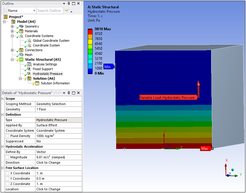
The following example shows the simulation of a Hydrostatic Pressure load on the wall of an aquarium. Here the wall is modeled as a single surface body. The load is scoped to the bottom side of the face. A fixed support is applied to the bottom edge. Acceleration due to gravity is used and the fluid density is entered as 1000 kg/m3. Coordinates representing the top of the fluid are also entered.
The load plot shown here illustrates the Hydrostatic Pressure gradient.
Details Pane Properties
The selections available in the Details pane are described below.
| Category | Property/Options/Description |
|---|---|
| Scope |
Scoping Method: This property specifies how you perform geometric entity selection. Options include Geometry Selection (default) and Named Selection. Geometry: Visible when the Scoping Method is set to Geometry Selection. Displays the type of geometry (Body, Face, etc.) and the number of geometric entities (for example: 1 Body, 2 Edges) to which the boundary has been applied using the selection tools. Named Selection: Visible when the Scoping Method is set to Named Selection. This field provides a drop-down list of available user–defined Named Selections. Shared Reference Body: This property is a scoping feature used to apply a Hydrostatic Pressure to shared faces or edges between two bodies. When you have properly scoped the geometric entities, using either Geometry Selection or an appropriate Named Selection, the property provides a drop-down list of the names of the bodies that share the scoped features. By selecting a body from this list, you are specifying that the pressure be applied to its surface or edge. Once selected, the Geometry or Named Selection property displays a parenthetical of the shared face or edge, "1 Shared Face/1 Shared Edge," to indicate the condition. Note:
Shell Face: This property enables you to specify the (default) or of the selected face. |
| Definition |
: Read-only field that displays boundary condition type - Hydrostatic Pressure. Applied By: This property defines how the load is applied. Either by creating surface effect elements or by direct application on the scoped geometry. Options include:
Coordinate System: Drop-down list of available coordinate systems. is the default. Suppressed: Include ( - default) or exclude () the boundary condition. Fluid Density: Input field for fluid density value. |
| Hydrostatic Acceleration |
Define By: Options include:
|
| Free Surface Location |
X Coordinate Y Coordinate Z Coordinate Location: Specify Free Surface Location using geometry picking tools. Valid topologies include face, edge, vertex. |
Mechanical APDL References and Notes
The following Mechanical APDL commands, element types, and considerations are applicable for this boundary condition.
When you set the Applied By property to Surface Effect, the Hydrostatic Pressure is applied as a surface load through the surface effect elements using the SFE command.
When you set the Applied By property to Direct, a Hydrostatic Pressure is applied directly on to the element faces using the SFCONTROL and SFE ,,PRES commands. Refer to SFCONTROL command for a list of supported solid elements, shell elements, and plane-2D elements.
Hydrostatic Pressure is represented as a table in the input file.
API Reference
For specific scripting information, see the Hydrostatic Pressure section of the ACT API Reference Guide.