


The Graph and Tabular Data windows enable you to review and modify the data, primarily associated with the objects and features listed below. When you select certain objects in the tree, the Graph window and Tabular Data window display beneath the Geometry window. Refer to the following topics for descriptions about the use of these windows as they relate to:
Analysis Settings
For analyses with multiple steps, you can use these windows to select the step(s) whose analysis settings you want to modify. The Graph window also displays all the loads used in the analysis.
These windows are also useful when using restarts. See Using Solution Restarts for more information.
Loading Conditions
Inserting a loading condition updates the Tabular Data window with an entry table that enables you to enter data on a per-step basis. The Graph window updates as you make Tabular Data entries.
All new tabular data is entered into the row that begins with an asterisk (*) regardless of whether the time or frequency point is higher or lower than the last defined point in the table. The application automatically sorts the content of the table into ascending order. In addition, any Tabular Data values preceded by an equal sign (=) are not defined table values. These values are application interpolated values shown for reference.
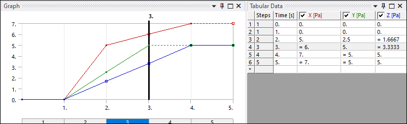
A check box is available in the column title for each component of a load in order to turn on or turn off the viewing of the load in the Graph window. Components are color-coded to match the component name in the Tabular Data window. Clicking on a time value in the Tabular Data window or selecting a row in the Graph window will update the display in the upper left corner of the Geometry window with the appropriate time value and load data.
As an example, if you use a Displacement load in an analysis with multiple steps, you can alter both the degrees of freedom and the component values for each step by modifying the contents in the Tabular Data window as shown above.
If you wish for a load to be active in some steps and removed in some other steps you can do so by following the steps outlined in Activating and Deactivating Loads.
Contour Results and Probes
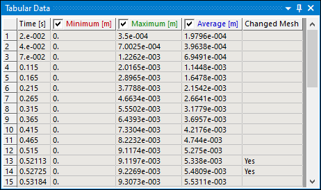
For contour results and probes, the Graph and Tabular Data windows display how the results vary over time. In addition, for result objects, the Tabular Data window usually displays the Total, as well as Minimum and Maximum values calculated on the specified geometry. The color of the column headers for these values corresponds to the colors displayed in the Graph window, red and green as illustrated below. You can animate your results in the Graph window for the specified result set domain. And, you can further specify a specific range to animate by dragging your mouse across graph content.
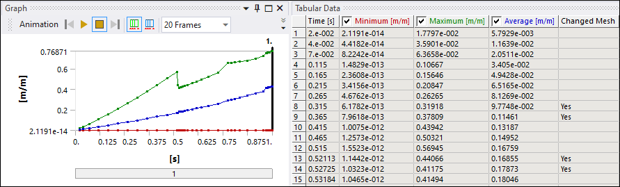
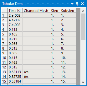
Note: If you refine the mesh using the Nonlinear Adaptive Region condition, the Changed Mesh column displays and indicates when mesh regeneration took place.
Important: For results displayed in the Tabular Data window, if
0 (zero) displays for both the Minimum and
Maximum values of a row, the result set may not contain result data.
You can use the option, discussed below, to view a
result set in order to determine if any data exists for the set. If no data is available,
the result contours in the Geometry window display as fully
transparent.
Retrieving Results
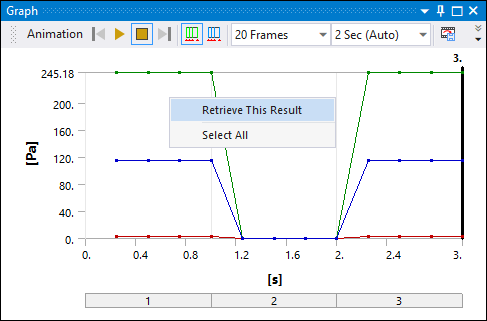
To view the results in the Geometry window for a desired time point, select the time point in the Graph window or Tabular Data window, then right-click the mouse and select . The Details for the chosen result object also updates to the selected step.
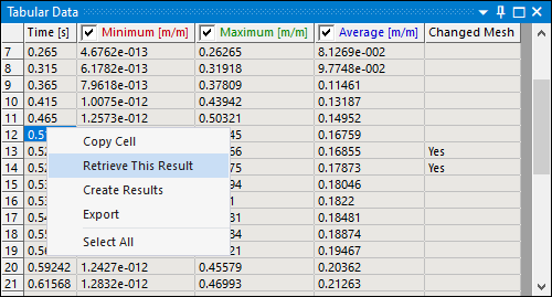
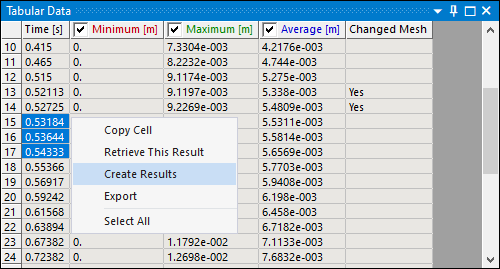
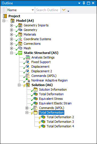
Creating Results
The contextual (right-click) menu of the Tabular Data window also includes an option to . This feature enables you to select multiple rows in the table and create individual results for each selection. These new results are placed in a Group folder in the tree. The Group folder has the same name as the original result. Or, in the event the originally result was already grouped, the new results are added to this existing group.
| Create Results Selection | Generated Results |
|
|
|
Display Graph Content in the Geometry Window
When the Geometry window has focus, you can select the Display Graph option on the Graphics Toolbar, or use the keyboard key G or the context (right-click) menu option, to display the content (load and result data) of the Graph window in the Geometry window. This enables you to include the graph in image captures of a viewport. Once displayed, you can drag and drop the graph within the window. You can activate this feature in multiple viewports and it remains active until you select one of the Display Graph options to remove the graph. In addition, the animation and animation export options support this feature.
Solution Steps and Substeps
During analyses that are using the Mechanical APDL solver, selecting the Solution object following the solution process for an analysis that includes multiple steps, the Tabular Data window displays the Time associated with each Step of the analysis as well as each Substep as applicable. The following examples of the Tabular Data window show these options for a deformation result.
|
Total Deformation Result Tabular Data
|
Solution Object Tabular Data
|
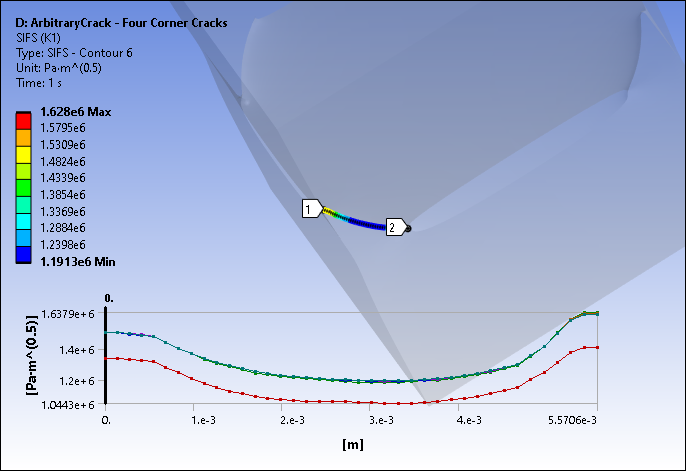
Charts
With charts, the Graph and Tabular Data windows can be used to display loads and results against time or against another load or results item.
Context Menu Options
Presented below are some of the commonly used options available in a context menu that displays when you click the right mouse button within the Graph window and/or the Tabular Data window. The options vary depending on how you are using these windows (for example, loads vs. results).
Retrieve This Result: As discussed above, for a selected object, this option retrieves and presents the result data at the selected time point you have selected in the Graph window or Tabular Data window.
Create Results: As discussed above, this option create result objects for the rows that you select in the Tabular Data window and places the new results in a group folder.
///: These options are available for Tabular Data content when the Solution object is selected for a solved analysis. These options enable you to create results for a selected row or multiple rows of data.
Insert Step: Inserts a new step at the currently selected time in the Graph window or Tabular Data window. The newly created step will have default analysis settings. All load objects in the analysis will be updated to include the new step.
Delete Step: Deletes a step.
Copy Cell: Copies the cell data into the clipboard for a selected cell or group of cells. The data may then be pasted into another cell or group of cells. The contents of the clipboard may also be copied into Microsoft Excel. Cell operations are only valid on load data and not data in the Steps column.
Paste Cell: Pastes the contents of the clipboard into the selected cell, or group of cells. Paste operations are compatible with Microsoft Excel.
Delete Rows: Removes the selected rows. In the Analysis Settings object this will remove corresponding steps. In case of loads this modifies the load vs time data.
Select All Steps: Selects all the steps. This is useful when you want to set identical analysis settings for all the steps.
Select All Highlighted Steps: Selects a subset of all the steps. This is useful when you want to set identical analysis settings for a subset of steps.
Activate/Deactivate at this step!: This enables a load to become inactive (deleted) in one or more steps. By default any defined load is active in all steps.
Zoom to Range: Zooms in on a subset of the data in the Graph window. Click and hold the left mouse at a step location and drag to another step location. The dragged region will highlight in blue. Next, select Zoom to Range. The chart will update with the selected step data filling the entire axis range. This also controls the time range over which animation takes place.
Zoom to Fit: If you have chosen Zoom to Range and are working in a zoomed region, choosing Zoom to Fit will return the axis to full range covering all steps.