This section provides step-by-step how-to instructions on the following topics:
- 4.4.1. Convert Between Crank Angle and Time
- 4.4.2. Specify, Change, or Specify Compression Ratio in an Engine Setup
- 4.4.3. Set Sub-Volume Region Initialization Order
- 4.4.4. Set Initial Swirl Ratio and Initial Swirl Profile
- 4.4.5. Set Up a Valve Lift Profile
- 4.4.6. Set Up a PFI Engine by Assuming Homogeneous Charge
- 4.4.7. Set Up a PFI Engine by Port Fuel Injection
- 4.4.8. Set Up a Gasoline Engine with Pre-chamber and Spark-Ignition
- 4.4.9. Model Knock
- 4.4.10. Speed Up a Flame Kernel Growth Under Lean-Burn Conditions for Gasoline Engines
- 4.4.11. Reduce Computational Time in Spark-Ignition (SI) Engine Simulation
- 4.4.12. Add or Modify Fuel Species in the Fuel Library
- 4.4.13. Set Up an Ammonia-Fueled Engine
- 4.4.14. Set Up a Hydrogen Combustion Engine
- 4.4.15. Monitor the Penetration Length of a Gas Injection Plume
To convert between a crank angle duration [degree] and a time duration [second] for a given rotation speed [RPM], use the following formulas:

To convert between a crank angle location [degree] and time location [second] for
a given rotation speed [RPM], assuming t = 0 aligns with
 , use the following formulas:

In Forte, you cannot directly input the compression ratio for the internal combustion engine. The value of the compression ratio is not needed/used in the calculation. Instead, the compression ratio is implied by the dimensions of the geometry such as the combustion chamber volume at piston Top-Dead-Center ("TDC") location and the dimensions of cylinder bore, stroke, connecting rod length, and piston offset.
In your Forte project, the compression ratio can be adjusted in different ways without requiring new CAD geometry, depending on what really happens in the engine hardware. Here are a few typical scenarios:
Adjust the Stroke value on the piston boundary condition panel. This input is available when you set the Motion Type of Wall Motion as "Slider Crank" in Wall Boundary Condition.
Adjust the squish height by moving the piston in the imported surface mesh. Note that the piston is at its TDC location when the surface mesh is imported. Therefore, adjusting the piston's location changes the squish height.
If the engine's simulation domain contains a volume representing the crevice region, adjust the height of the crevice region.
There is a Compression Ratio Calculator in the Forte UI (Compression Ratio Calculator in the Ansys Forte User's Guide), which can be used to calculate and verify the compression ratio based on the previously mentioned geometric parameters. Note that in this calculator, all the valves are forced to be seated when the Bottom-Dead-Center ("BDC") and TDC volumes are calculated.
Initialization order is important when using sub-volumes for initial conditions: the rule is that sub-volumes must be applied before material point regions (the global initialization counts as a material point-based region for this purpose) and so setting initialization order to 1 for the sub-volume and 2 for the default region works as expected.
The definition of swirl ratio can be found in Spatially averaged variables that are always output to the .csv files in the Ansys Forte User's Guide. A detailed description of the initial swirl profile can be found in Swirl Profiles in the Ansys Forte Theory Manual.
Both swirl ratio and swirl profile are mainly dependent on the intake manifold configuration or intake valve timing. For example, swirl can be created by using a swirl valve in the intake manifold, using a special spiral shape of intake manifold, or using different valve lift profiles for two intake valves. These swirl-generating devices can be used in any types of engine. The detailed settings are dependent on the specific engine configuration.
The initial swirl settings are important for a closed cycle simulation, in which the intake stroke is not part of the simulation and these swirl settings at IVC are empirically set. If the initial swirl ratio is completely unknown and the engine is likely to have a strong swirl, the best practice is to carry out a full cycle simulation (by including the intake stroke simulation) and compute the initial swirl at IVC, and then the computed IVC swirl ratio can be used to initialize the closed cycle simulation. Alternatively, the velocity solution at IVC in the full cycle simulation can be used to initialize the velocity field in the closed cycle simulation through IC (initial condition) table lookup.
In a full cycle simulation, if the simulation starts before IVO, the initial swirl settings typically have very small impact on the results because the initial velocity pattern inside the cylinder is likely to be flushed out and overridden by the intake flow. The initial swirl settings are even less important in a multicycle simulation.
For setting up a valve lift profile, a typical valve motion activation threshold is set between 0.2 mm and 0.3 mm, with approximately 1.5 to 2 cells in the gap at the minimum lift. Use the Valve Lift utility to add an opening/closing step to the profile and the Check Valves utility to make sure the valves are in a closed position. Also, with a 2 mm global mesh size, apply a ¼ refinement to the bottom part of the valves.
Typically, in PFI gasoline engines, the mixing between intake charge and fuel creates a nearly homogeneous mixture before a spark occurs. If the global equivalence ratio is known, it is an acceptable approximation to use a premixed homogeneous mixture directly instead of including the port fuel injection. In this case, the intake manifold can be initialized using the premixed air/fuel mixture and the same mixture can be used as the boundary condition at the inlet. The cylinder and exhaust manifold can be initialized as a completely combusted mixture. Such a setup will automatically consider the internal EGR (also called internal residual). If there is external EGR, it should be considered in the premixed air/fuel mixture. The IVC composition calculator utility in Forte can be used to compute all these different mixture compositions.
When including port fuel injection in the simulation for PFI engines, make sure the initial droplet size does not use the uniform size option, instead, use the Rosin-Rammler distribution with SMD around 10–15 micron. Also, it may be worth doing a multicycle simulation to eliminate uncertainty associated with the initial condition.
While there is no specific example for a prechamber gasoline engine with spark ignition, it can be set up following the best practices for a generic gasoline engine with spark ignition (Setting Up Generic Engine Cases with Valve Motion Using Automatic Mesh Generation).
One difference would be how to initialize the pre-chamber. This is left to your preference. The prechamber could be initialized as a single domain together with the main cylinder. Alternatively, a prechamber sub-volume could be created at the Geometry node level and used as a different initialization region at the Initialization node level. Note that if the second approach is preferred, the initialization order of the pre-chamber must be smaller than that of the main cylinder. For more information about the initialization order, refer to Initialization Order.
Another difference is in the surface-based mesh refinement settings. While we recommend ½ refinement for wall boundaries and open boundaries in general, we might need ¼ refinement at the walls of the pre-chamber and need ¼ or even ⅛ refinement at the open boundaries connected to the pre-chamber, mainly because the size of the pre-chamber is typically smaller than that of the main cylinder.
Modeling methodology
Knock occurs in spark ignition engines due to autoignition in the end gas zone ahead of flame arrival. Forte uses the G-equation model to simulate turbulent flame propagation. Detailed chemical kinetics is solved everywhere inside the combustion chamber using the Chemkin solver. In the flame front zone, chemical heat release is also solved by the flame propagation model, where the mixture swept by the mean flame front surface is assumed to reach local and instantaneous chemical equilibrium. Typically, the heat release rate from the flame propagation model is much larger than that from the autoignition kinetics, and therefore combustion is mainly driven by flame propagation. However, if the end gas temperature becomes high enough due to compression, auto-ignition may occur. Stronger autoignition in the end gas zone leads to stronger knock intensity.
Chemistry for autoignition kinetics
The detailed chemistry mechanism used for knock modeling must contain low temperature kinetics. A rich set of pre-reduced chemistry mechanisms for various fuels are supplied in the Ansys installation. Most of these mechanisms can be used for knock modeling, but some of them are reduced for high temperature combustion applications only, so pay attention to their valid pressure and temperature ranges. These mechanisms can be found in the data folders under either reaction or forte. For example, in the Windows installation, these folders are:
\reaction\data
\reaction\forte.win64\data
The details of these mechanisms are described in Model Fuel Library Getting Started Guide and Forte User's Guide (Appendix D).
Below are some notes specific to gasoline combustion and natural gas combustion:
Gasoline
Before setting up the simulation project, check what is the intended octane number (ON) of the fuel used in the engine being modeled. Isooctane (iC8H18) is a good surrogate for modeling flame propagation speed and heat release rate, but its ON rating is 100 and consequently it may have larger knock resistance than most of the gasoline fuels sold at the pump. If the actual fuel's ON is lower than 100, it will make sense to use a multi-component fuel surrogate to match the intended ON value.
The simplest option for modeling an ON < 100 fuel is to use a primary reference fuel (PRF), which is a mixture of isooctane (ON=100) and n-heptane (ON=0, nC7H16). For example, PRF87 (ON=87) consists of 87% isooctane and 13% n-heptane by volume.
You can also consider using a TRF fuel (toluene + isooctane + n-heptane) to model the impact of aromatics. One example TRF surrogate from our previous study for ON91 fuel is:
ON 91, mass % C6H5CH3 21.5% iC8H18 65.0% nC7H16 13.5% Another option is to use the Surrogate Blend Optimizer (SBO) in Chemkin to generate a surrogate blend based on the actual fuel's ON and other properties. To use SBO, refer to:
After you have determined the composition of the fuel surrogate, you can select a suitable pre-reduced mechanism from the data folders mentioned above.
Natural gas
Natural gas can be modeled as a single component (CH4) fuel or a multi-component mixture. A suite of natural gas mechanisms pre-reduced from the MFL master mechanism is available in folder:
\reaction\data\ModelFuelLibrary
Decision flowchart for selecting MFL natural gas mechanism in the Model Fuel Library Getting Started Guide provides a clear guide on selecting MFL natural gas mechanisms.
For knock application, the single component mechanism naturalGas_methane_MFL2020.cks should not be used because it does not contain low temperature autoignition kinetics. Similarly, the single-component mechanism NaturalGas_1comp_29sp.cks in folder \reaction\forte.win64\data should not be used for the same reason.
To model natural gas as a single component fuel for knock application, you can consider using the GRI3.0 mechanism as well, which is available in the \reaction\data folder.
One note related to laminar flame speed input: if the fuel surrogate mixture is modified, and if you are using the Table Library option for laminar flame speed (Models > Chemistry > Flame Speed Model), remember that the composition of the laminar flame speed library may need adjustment to match the updated fuel surrogate composition.
Another model to mention here is the AIF (Autoignition Induced Flame Propagation) model, which can be found on the Simulation Controls > Chemistry Solver panel. The AIF model is designed for initializing flame propagation without spark ignition. Its typical application is dual fuel engines in which pilot diesel fuel is injected into a premixed mixture of air and a second fuel. This model is not related to knock modeling and should remain turned off in knock applications.
Solution monitoring and post-processing
Knock can be monitored and analyzed in three different ways in Forte:
Use monitor probe to monitor local pressures
When knock occurs, the resulting pressure wave could cause large fluctuations to pressures monitored at selected locations in the combustion chamber. To mimic pressure transducers used in experimental measurement, you can use Monitor Probes in Forte simulation to monitor local pressure.
The monitor probes can be placed at several locations near the liner and below the cylinder head. You may add as many monitor probes as needed along the periphery of the cylinder head. The pressure fluctuation characteristics could be quite different at different locations. Note that the fluctuating pattern is hard to notice on the cylinder-averaged pressure trace.
The pressure wave relevant to knock is typically in the range of 3 to 15 kHz. To capture these waves on the local pressure curves, a high sampling frequency is needed. The maximum CFD time step size should be sufficiently small (on the level of 5.E-7 s or smaller) during combustion and the early stage of the expansion stroke. The data saving interval of the monitor probes should be equal to or smaller than the CFD time step size.
You can use your own data processing tool to post-process the raw pressure data sampled through the monitor probes. Forte Monitor also provides a high pass Butterworth filter for filtering out the low-frequency components. To use this Butterworth filter, right-click the pressure variable shown on the variable list in Forte Monitor and click Apply Filter.... The Cut off is a non-dimensional parameter calculated as
 . For example, if
  is 5.E-7 s and the
  is 3.E3 Hz, the Cut off should be
0.003.
is 3.E3 Hz, the Cut off should be
0.003.Check chemical heat release from different combustion zones
Starting from Release 2021 R2, chemical heat release rate and accumulated chemical heat release from three different combustion zones are reported in flame.csv. The three zones are flame front zone, end gas zone, and post flame zone. These outputs can be used to monitor how much heat is released in the end gas zone due to auto-ignition. If a significant amount of chemical energy is released from the end gas zone, the knock propensity of this condition is high.
Visual inspection of high temperature spots in the end gas zone
After loading in the spatially resolved solutions into EnSight, you can monitor whether any autoignition occurs in the end gas by creating a G=0 iso-surface and checking whether there are high temperature spots on the end gas side. When setting up the output controls, make sure Temperature and G are selected as spatially resolved outputs. You should also consider using user-defined output crank angles to save spatially resolved solutions (.ftres) at relatively higher frequency during the flame propagation phase to get higher time resolution of the solutions.
The following are a list of settings that can help in speeding up a flame kernel growth:
For Laminar Flame Speed, use the Table Library option.
For Turbulent Flame Speed, set the Stretch Factor Coefficient to 0.
For Unburned Calculation Method, use the Volume Search with Variable Radius option.
Make sure the mesh in the spark plug region is sufficiently refined such that the initial spherical flame kernel structure can cover at least 2-3 layers of cells along its diameter.
The Turbulent Flame Speed Ratio (b1) in Turbulent Flame Speed and the Flame Development Coefficient on the Spark Ignition" panel are two model constants that can be adjusted (increased) to speed up flame propagation. Such adjustment is sometimes needed to account for uncertainties in turbulence solution field.
The following are some tips that may reduce the computational time:
Certain cases, especially those with a large intake port, could benefit from a larger global mesh size. Larger global mesh size can save some cell count at places where mesh resolution isn't that important. At the same time, you might want to maintain the desired mesh resolution in some local spots (for example, around the valve surfaces) by deepening their mesh refinement levels. To maintain the resolution of physics, you could use a Solution Adaptive Mesh (SAM) refinement based on VelocityMagnitude and G.
In Simulation Controls > Chemistry Solver, it is recommended to activate chemistry only between the start of spark ignition and the EVO, such as from 693 deg to 837 deg. Note that this crank angle range is for the primary cylinder. It will be automatically applied with respect to the second cylinder's local time frame.
In Simulation Controls > Chemistry Solver, you could turn on Use Species Lumping When Chemistry is Deactivated. The main benefit is to reduce the computational cost of transporting many species with flows. The tooltips and Forte User's Guide have guidance on how to set the Core Species and Absorbing Species. In an old Forte project, you might have to manually pick the relevant species according to the guidance. Usually when starting with a new Forte project and importing a chemistry mechanism, the default Core Species and Absorbing Species are automatically populated.
The max flow velocity (in flow_diagnostics.csv) could be rather large when the exhaust valves open. This reduces the time step. Make sure to add stepping at the opening and closing of the valve in the valve lift profile. You can turn on Solution Constraints on Velocity and Mach Limit under Simulation Controls to see if they are helpful.
In Models > Chemistry/Materials > Chemkin Chemistry Set > Flame Speed Model, make sure that the Disable Flame Propagation Model option is set as the default option When an Engine Cylinder is not a closed system. It is better not to keep solving the flame propagation model when the cylinder has been connected to the port regions.
To add new fuel species or modify the properties of existing fuel species in the fuel library, you must modify the fuel_library.inp in the data folder of the Forte installation. This library is shared by all Forte projects using this Forte installation. After modifying this file, reload the Forte Simulate UI, and the modified fuel library will be picked up by the UI automatically. The modified species list will show up on the spray composition setup panel.
When the Nominal/Run folders are prepared, the Forte UI will duplicate the fuel_library.inp file in the Nominal/Run folder and rename it as fuel_lib_chem.inp, which is used as the input for forte.exe.
Since the .ftsim file identifies fuel species by their indices as listed in the SPECIES list, to avoid affecting old projects, the best practice is NOT to modify the order of the existing species list or their properties. Instead, you can duplicate an existing species, give it a different name, append it to the end of the SPECIES list, and duplicate (and modify) the properties. Below are the detailed steps of adding a new species:
Add the new species name to the end of the list in the SPECIES block.
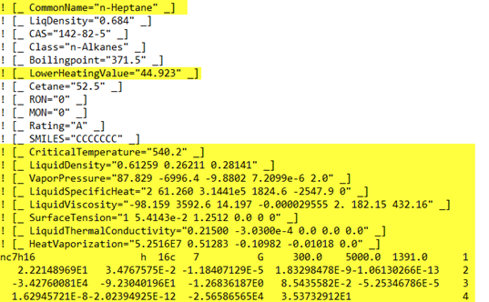
Include the properties listed below in the THERMO block (n-heptane is used as an example here). Note that each block starts with the "CommonName" item and ends with the thermodynamic data coefficients. The highlighted items are required. For the details of the property correlations, refer to Fuel Library in the Ansys Forte User's Guide.
Add transport data for the new species in the TRANSPORT block. (Note: Chemkin Reaction Workbench can be used to estimate many of these properties.)
To check for errors in the modified fuel_library.inp, import the fuel_library.cks chemistry set into the Forte Simulate UI and run the pre-processing utility (the same procedure as importing a gas-phase chemistry set) and see if any error is reported in the output file. Note that this error check step is optional. If Forte Simulate UI complains that the newly added species cannot be found, double check the properties for typos—for example, the CommonName entry may be missing the double quotes.
There are different ways ammonia is introduced into engines as fuel depending on the engine configuration and the specific ammonia solution being used.
For injection of liquid ammonia solution, it is assumed that the liquid being injected is ammonium hydroxide (NH4OH). This liquid breaks down into NH3 and H2O at around 38°C. Instead of treating NH4OH -> NH3 + H2O as a chemical reaction, the injected fuel can be approximated as a two-component mixture, NH3 and H2O. The tricky part is how to specify a liquid fuel species that can be mapped to NH3. Note that NH3 and H2O need to be mapped to different fuel species in the fuel library in the fuel injection setup. H2O is already in the fuel library, but a "fuel" species must be added in the fuel library for NH3. If the ambient temperature is very high (well above the boiling temperature of water) when ammonia injection occurs, it may be ok to use the physical property of H2O or a fuel that is more volatile.
The new fuel species for NH3 should be added to the fuel_library.inp file in C:\Program Files\ANSYS Inc\v***\reaction\forte.win64\data. You can start by duplicating species H2O, renaming it as NH3, replacing the thermodynamic coefficients by those of NH3, and adjusting the liquid properties to make it more volatile. Once the fuel_libary.inp is modified, you need to reload Forte Simulate UI to make the new species show up. Some research is needed here to come up with the approximated "liquid" properties for NH3, which is essentially gas after coming out of NH4OH.
If the injection occurs upstream in the intake manifold for creating premixed fuel/air mixture, NH3 can also be introduced into the system through a gas inlet boundary in the simulation.
For pure hydrogen combustion, it is recommended to use our latest published mechanism (first available in 2022 R1) over GRI-mech. The skeletal versions (one with NOx and the other without NOx) can be found in the Ansys installation: C:\Program Files\ANSYS Inc\v221\reaction\data\ModelFuelLibrary\Skeletal. This mechanism is open-source and extracted from the larger Gaseous C0-C6 mechanism.
The publication can be found in the following link:
In addition, it is recommended that you follow these best practices:
For the Flame Speed Model, for the Laminar Flame Speed option, use the Table Library option (instead of the default Power Law) and add h2.
Set b1 to 3.
For Spark Ignition, set Min. Kernel Radius for Kernel to G-equation Switch to 1 mm. However, if slow from DPKM to G-equation use 2 mm, as the larger kernel size helps to move away from the kernel stage.
Use restart before spark.
Increase the number of parcels to 30000 from 3000.
Forte currently does not have a dedicated utility for monitoring the penetration length of a gas injection plume. Although EnSight can be used to derive this output information, it requires spatially resolved solutions to be saved at high frequency, which may not be desirable. As a workaround, the spray penetration length analysis utility can be "borrowed" to serve this purpose. This approach requires creating a liquid-spray injector that serves as a helper and is never activated. Here are the steps with H2 injection as an example:
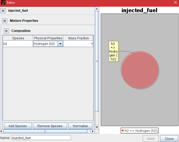
Under Models > Spray Model, add a solid cone injector. For the Composition of the "injected" mixture, add h2 as the Species and map it to Hydrogen (h2) in the fuel library (as shown in Figure 4.28: Composition editor specifying the injected mixture), and set its mass fraction to 1. For all the other required input parameters on this injector setup panel, give them arbitrary (but ideally still physical) values. These values won't be used.
For this solid cone injector, add a nozzle and an injection. On the nozzle panel, all the inputs can be set to arbitrary values because they won't be used, but make sure the spray direction vector is not a zero vector in order to pass the error check. On the Injector panel, for either CA-based or time-based timing, set the start of injection to be a value much later than the "End of Simulation" time. The purpose is to make sure this start of injection time will never be reached and this spray model will never be activated. Simply pick the Square Profile as the injection profile and use any positive value for the total injected mass.
To set up the penetration output, in Output Controls > Spatially Averaged And Spray, at the top of this panel, click the New penetration analysis
 icon to add this Penetration
Length option. On this Penetration Length panel, select
Injector as the Spray Source
option, choose the Solid cone injector from the
Injector list. Now, define the origin and the axis of the injector to match
the configuration of the H2 gas injection. Change the Vapor
Penetration Length Threshold from the default value of 0.99 to a
smaller value, such as 0.9999.
icon to add this Penetration
Length option. On this Penetration Length panel, select
Injector as the Spray Source
option, choose the Solid cone injector from the
Injector list. Now, define the origin and the axis of the injector to match
the configuration of the H2 gas injection. Change the Vapor
Penetration Length Threshold from the default value of 0.99 to a
smaller value, such as 0.9999.In the simulation, the "vapor" penetration length will be reported in a .csv file called custom_spray_penetration.csv. This vapor penetration length measures how far the H2 cloud reaches along the injector axis direction defined in step 3, with respect to the origin of the injector (also defined in step 3).