Begin by selecting the Surrogate Blend Optimizer from the Workbench  , or by loading the Surrogate Blend Optimizer project located in the
samples<release_number> directory, where
samples<release_number> is something like
samples2021R1. Set up the working directory, the chemistry
set.
, or by loading the Surrogate Blend Optimizer project located in the
samples<release_number> directory, where
samples<release_number> is something like
samples2021R1. Set up the working directory, the chemistry
set.
The recommended input files for the chemistry set are in the samples<release_number>/ surrogate_blend directory and the surrogate blend sample, surrogate_blend.ckrsg, is in the samples<release_number> directory. It contains references to an example set of input parameters.
In the example illustrated here, the gasoline mechanism was tagged to include the following fuel species:
c5h10-1, ic8h18, nc7h16, c6h5ch3, and mch
For this example, we choose to model a gasoline blend with the following fuel properties.
Table 2.1: Components and properties of gasoline blend
|
Component class |
Target liq. vol. frac. |
Approximate range of variation |
|---|---|---|
|
Alkenes |
5 |
1 – 8 |
|
Cycloalkanes |
10 |
1 – 10 |
|
Aromatics |
25 |
10 – 45 |
Table 2.3: Selected points from typical boiling point curve (based on ASTM D2887 method)
|
Distillation Curve Point |
Temperature (K) |
Acceptable range of temperature variation for testing (K) |
|---|---|---|
|
T10 |
324 |
±50 |
|
T50 |
368 |
±10 |
|
T90 |
422 |
±50 |
Fuel components selected for the surrogate blend should include one or more components for each major chemical class present in the real fuel. For gasoline, the selected component can within a carbon number range of 4 to 12, and for diesel it can be from 9 to 24 [2]. Selection of the components also depends on the targets. Select components so they bracket the property values of the targets. Table 2.4: Selected fuels lists fuels chosen in this tutorial. The components cover all the major chemical classes in gasoline and cover the range of target values listed in Table 2.2: Target properties for components in gasoline blend and Table 2.3: Selected points from typical boiling point curve (based on ASTM D2887 method). Additional components would be required if more points from the distillation curve are included as targets.
Table 2.4: Selected fuels
|
Fuel Class |
Species Name |
Fuel Name |
|---|---|---|
|
Alkenes |
c5h10-1 |
1-Pentene |
|
Aromatics |
c6h5ch3 |
Toluene |
|
Cycloalkanes |
mch |
Methylcyclohexane |
|
iso-Alkanes |
ic8h18 |
iso-Octane |
|
n-Alkanes |
nc7h16 |
n-Heptane |
The next step is to specify the fuel property targets.
This result is fast, and it shows that the fuels chosen can reasonably represent the required fuel properties.
Summarized below are results of a quick calculation of composition matching to distillation curve, lower heating value, hydrocarbon ratio, and several fuel classes.
Table 2.5: Calculated gasoline surrogate composition
|
Species |
Liquid Volume % |
|---|---|
|
1-Pentene |
06.89 |
|
Toluene |
024.96 |
|
Methylcyclohexane |
009.50 |
|
iso-Octane |
046.87 |
|
n-Heptane |
011.78 |
The high discrepancy at the T90 results indicates that achieving a value of 422 is not possible given this set of surrogates. To improve the applicability of the surrogate, we also add styrene, which has a pure component boiling point of 419 K.
This results in an improvement in the distillation curve.
This tutorial demonstrates the capabilities in Reaction Workbench for targeted mechanism reduction. While Ansys Chemkin mechanisms cover a large number of surrogate fuels and blends and include very comprehensive chemistry in terms of ranges of combustion conditions, the direct use of the mechanisms in engine simulations is impractical, due to the mechanism size. The mechanisms, then, must be reduced as needed for the application of interest. In this tutorial, we demonstrate the reduction of an 1883-species full mechanism to a 134-species reduced mechanism, focusing on accurately capturing n-heptane chemistry; the single component n-heptane surrogate is used to represent diesel combustion chemistry.
This tutorial highlights the following aspects of the Reaction Workbench mechanism reduction process:
Definition of operating range: Specify the operating conditions of interest, such as temperature, pressure, equivalence ratio and dilution. In this sample, a parameter study of 8 cases varying temperatures from 700–1150 K and equivalence ratios from 1–3 is considered to account for a range of these conditions.
Definition of success criteria: Define the success criteria for the mechanism reduction. This involves defining "targets" of interest, such as ignition times and emitted species concentrations, and the degree to which predictions for these targets with the reduced mechanism should match with the predictions made with the full mechanism.
Choice of reduction technique: Decide the sequence of reduction techniques to use. Reaction Workbench offers the following reduction techniques. This tutorial highlights how Reaction Workbench facilitates the use of any combination of these techniques.
DRG (Directed Relation Graph)
DRGEP (Directed Relation Graph with Error Propagation)
DRGPFA (Directed Relation Graph with Path Flux Analysis)
Sensitivity Analysis Option in DRG/DRGEP/DRGPFA
PCA (Principal Component Analysis)
QSSA (Linearized Quasi-Steady-State Approximation)
Linear lumping of isomer species
FSSA (Full Species Sensitivity Analysis)
Automation and Decision Making: Reaction Workbench automatically creates and tests reduced mechanisms as they are created, until the optimal reduced mechanism is generated. At the end of the sequence of reduction steps you can decide the next step to take and/or archive the current "optimal" mechanism.
In this sample we focus on n-heptane as the fuel, which is frequently used as a 1- component diesel surrogate. The goal is to generate a reduced mechanism for n-heptane that is as small as possible while maintaining our specified level of accuracy over the desired range of operating conditions. We use the 14-component diesel surrogate mechanism (diesel_14comp.cks) as the full mechanism for this project: this mechanism has the requisite n-heptane chemistry pathways of interest.
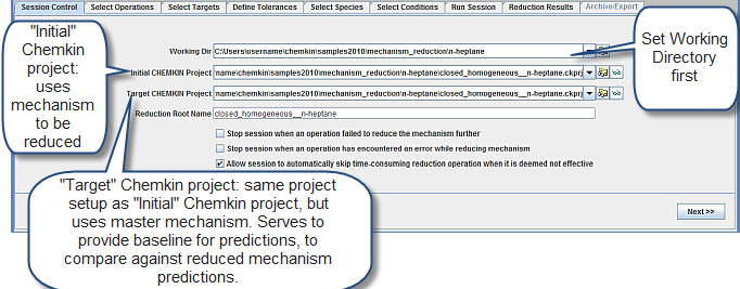
The mechanism reduction project file is mechanism-reduction__n-heptane.ckmrs in samples<release_number>/ (in your chemkin directory). The working directory is samples<release_number>/mechanism_reduction/n-heptane. Once the file is opened in Reaction Workbench, the first panel in the Reaction Workbench mechanism reduction user interface is the Session Control panel, as shown in Figure 2.3: Session Control panel in the Mechanism Reduction utility. The first action in this panel is to set the Working Directory (pre-set in this example).
Next, Ansys Chemkin projects must be defined (also pre-set in this sample). The Chemkin project is used to solve the relevant engineering problem. It is typically set up as a parameter study, in which parameters are varied to cover the range of conditions of interest for an engineering simulation. For Chemkin simulations, the project is usually a 0-D simulation, where the kinetic timescales are representative of the real system and the parameter study is used to represent stratification of combustion conditions, such as temperature and equivalence ratio. The baseline project serves two purposes:
The mechanism reduction techniques use the solution of this Ansys Chemkin project to perform the reduction.
Once reduced mechanisms are generated, the predictions from this Ansys Chemkin project will be used to evaluate the accuracy of the reduced mechanism, by comparison with the full mechanism predictions, for "targets" of interest (such as ignition time and emission species).
In Figure 2.3: Session Control panel in the Mechanism Reduction utility, two Ansys Chemkin projects are requested, the Initial and the Target Chemkin projects. Both of these are expected to have the same project setup, except for the mechanism used. The Target Chemkin project uses the full mechanism, and predictions using this project form the baseline against which reduced mechanisms will be evaluated. The Initial Chemkin project uses the mechanism that must be reduced. In the first reduction step, the Target and Initial Chemkin projects are the same, both using the full mechanism. However, later in this tutorial, follow-up mechanism reduction operations will be used for further reduction. In those operations, the Initial and Target Chemkin projects will be different, with the Initial project using the reduced mechanism from a previous operation.
The choice of the Ansys Chemkin reactor model used in the Target project depends on the engineering problem of interest. Workbench allows any Chemkin model to be used for mechanism reduction. The Chemkin Batch reactor model is appropriate for most reduction cases. For ease of setup, a Batch reactor template can be used when performing mechanism reduction, where only the operating conditions need to be specified. In this tutorial, we are using the Batch reactor template to create a reduced mechanism for compression-ignition engine conditions. In a compression-ignition engine with fuel injection, the local equivalence ratios and temperatures are expected to be quite stratified. For the purposes of reducing the mechanism, the geometry, spray and turbulence effects do not have to be simulated directly. It is, however, important to consider the range of local operating conditions such as temperatures and equivalence ratios that result from these effects, when defining the reduction targets. A range of initial temperatures and equivalence ratios are specified in the batch-reactor Chemkin project, through the use of a parameter study. This allows the 0-D model to be used to represent the local stratified conditions in the engine:
Initial equivalence ratios of 1–3.
Initial temperatures of 700–1150 K.
Initial pressure of 50 atm. This pressure was chosen as indicative of pressure close to TDC, where ignition occurs.
Note: Reduction Root Name can be used to specify the root name of the reduction files, and therefore provide clarity in file and folder names. For instance, if the root name is n-heptane, after the drgep001 reduction is completed, those files and folders will be named n-heptane_drgep001. Note that there is a limit of 256 characters for the path to files, so ensure that the reduction root name is not too long.
Next, in the Select Operations panel, the sequence of reduction techniques to be used can be specified. Depending on the full mechanism size and other setup details, a sequence of techniques are pre-populated as a good starting point. As appropriate, this sequence of techniques can be modified or more techniques can be added to the end of this pre-populated list. Figure 2.4: Select Operations panel in the Mechanism Reduction utility provides the sequence of reduction operations for this sample.
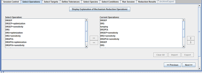
Note: The PCA reduction technique will not be listed as an option in the Select Operations panel, using this sample. This is because the Ansys Chemkin project used in this sample does not include reaction-rate sensitivity analysis. If the PCA technique is desired, the Chemkin project must be modified to include sensitivity analysis.
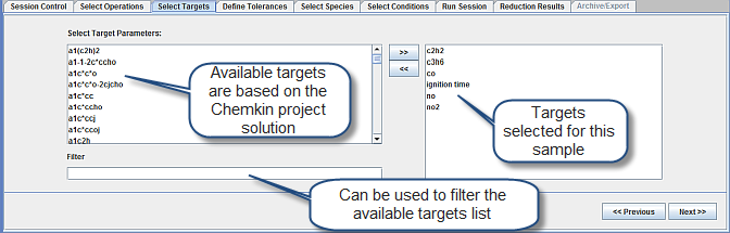
Once the Ansys Chemkin projects and reduction technique have been specified, we move to the Select Targets panel, shown in Figure 2.5: Select Targets panel for the Mechanism Reduction utility. This panel and the next help define the success criteria for mechanism reduction. The Workbench performs a series of mechanism reductions that gradually get more aggressive. It is important that you define criteria by which these series of mechanisms can be evaluated. In this sample, the targets selected are:
Ignition times
Emissions-related species:
NO, NO2
CO
C2H2 (representative soot-precursor)
C3H6 (representative unburned hydrocarbon species
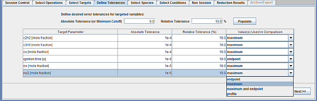
In the next panel, Define Tolerances, you set criteria for how well the predictions for the targets using the reduced mechanism should match those using the full mechanism. This is specified using absolute and relative tolerances for each target. The panel is shown in Figure 2.6: Define Tolerances panel for the Mechanism Reduction utility. The way the absolute and relative tolerances are used is defined in Chemkin Reaction Workbench User's Manual, in the discussion of "Controlling Target Error in Skeletal Mechanisms." This sample specifies non-zero values for both absolute and relative tolerances. This way, the absolute tolerances are effectively used to filter out very small values that do not merit interest: ignition times below 1 microsec, emissions below 100 ppm for CO, propene, and acetylene, and 10 ppm for NO and NO2 are ignored when comparing the full and reduced mechanism predictions. The relative tolerances are set to 10% for all targets. These tolerance values are based on the guidance in the Mechanism Reduction Best Practices, available on the Ansys Help website.
Note that the "Values used for comparison" column in Figure 2.6: Define Tolerances panel for the Mechanism Reduction utility for this sample uses maximum values for acetylene, CO and NO, and end-point for ignition times. There are three options in this column that you can select, as shown in Figure 2.6: Define Tolerances panel for the Mechanism Reduction utility.
The first option, the profile, is the most stringent. For the case of the acetylene target, for instance, for each time point in the profile, the acetylene predictions from the full and reduced mechanism are compared to see if they match within the specified tolerances. So, even though the profile shapes might match qualitatively, if there is a slight shift in the profiles on the order of tens of microseconds, it could potentially violate the user-specified tolerances for some of the time points.
The second option, which is less stringent, compares the end-point values only (the values at the end time), when comparing the full and reduced mechanism predictions.
The third option, also less stringent than option 1, compares the maximum point values only, when comparing the full and reduced mechanism predictions. It does not matter if the maximum values are reached at different time locations. In this sample, for all the emission-related species, the maximum option is chosen. This does not guarantee that the trends of species profiles using full and reduced mechanisms would match, and it is a good idea to check these profiles for a few cases manually after mechanism reduction.
Note: For demonstration purposes only, this sample was run using only the last ignition time as the target (that is, for cases with multiple ignition times, use only the last value as target). This was set under Edit > Preferences, and checking the Use Last Ignition Time as Target Parameter check box. If this setting is not used, the more stringent condition of using all ignition-time values as targets will be employed.
In general, as more accuracy is sought from the reduced mechanism, the size of the reduced mechanism increases. You can control this balance between accuracy and size of the reduced mechanism using the number of targets defined and the accuracy sought for those targets.
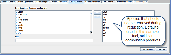
In the Select Species panel shown in Figure 2.7: Select Species panel for the Mechanism Reduction utility, the defaults are used for species that should not be removed during mechanism reduction: fuel, oxidizer, combustion products, and the targets.
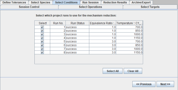
Next, in the Select Conditions panel, all the eight parameter studies covering 700–1150 K and equivalence ratios of 1–3 that were defined in the Ansys Chemkin project are selected. So, the reduced mechanism would be valid for all these conditions.
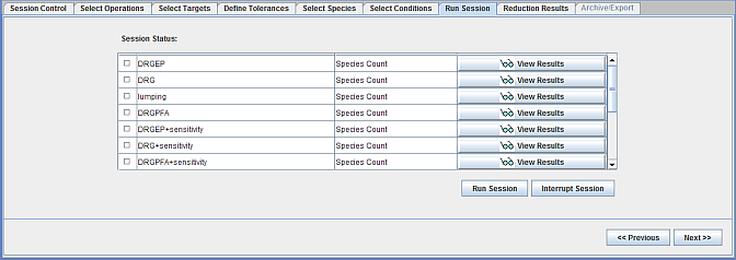
Next, in the Run Session panel, the Session can be started and interrupted. Results of a particular reduction can be viewed using the View Results icon. Figure 2.9: Run Session panel in the Mechanism Reduction interface shows the Run Session panel.
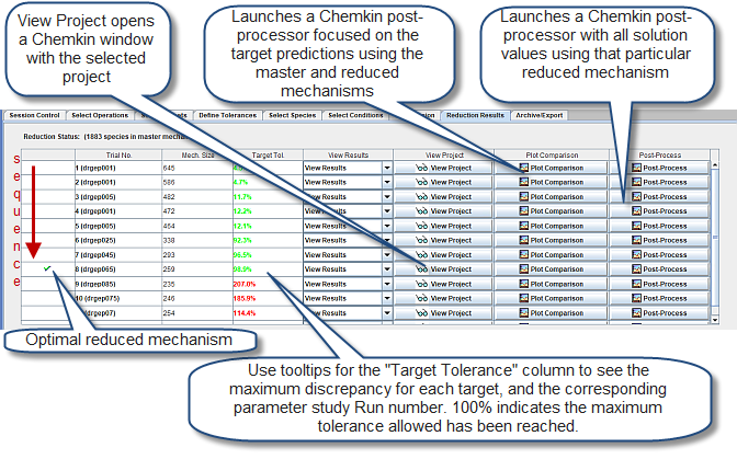
Finally, in the Reduction Results panel, the results of any reduction operation can be viewed. Figure 2.10: Reduction Results panel for the Mechanism Reduction utility shows the results after the mechanism reduction operation is finished for a DRGEP operation. A series of reduction runs are performed automatically, gradually getting more aggressive. Reductions that exceed user-specified tolerances are rejected. Rejections are highlighted in red in the panel, for instance Trial 4. In this sample, DRGEP is used. All of the trial runs are performed in an automatic fashion, so as to generate the smallest mechanism possible while obeying user-specified tolerances for the targets specified. The Plot Comparison option shown in the figure provides a visual understanding of how well the full and reduced mechanism predictions compare. The "Target Tol." column shows the maximum discrepancy for that trial, relative to user-specified tolerances; a value of 100% indicates the maximum user-specified tolerance has been met. Since parameter studies are involved in this sample, seeing the bubble help for the numbers in the "Target Tol." column is useful, as it shows the maximum discrepancy for each of the targets, and the parameter-study Run number associated with this maximum discrepancy.
The sequence of reduction techniques yielded a 134-species reduced mechanism. Beyond a certain point, further reductions do not yield substantial returns on the mechanism reduction. In this sample, DRG, DRGEP, DRGPFA, isomer lumping, and species sensitivity analysis techniques were used. Additional reduction techniques are also available in Reaction Workbench.
Note: DRG and DRGEP are among the computationally fastest and most efficient reduction techniques. These are the workhorses for reduction, especially for large mechanisms. Species sensitivity analysis techniques (both DRG- and DRGEP-based) are time-intensive, and so best used near the end of the reduction (that is, on smaller, reduced mechanisms).
This 134-species mechanism matches all targets within the user-specified tolerances (see Figure 2.6: Define Tolerances panel for the Mechanism Reduction utility for original user-specified tolerances). Note that if tolerances are relaxed or the parameter studies are run with narrower ranges of temperatures or equivalence ratios, further reduction is possible.
As demonstrated in this tutorial, the use of several reduction methods through iterative reduction operations can be more effective than using a single method. Table 2.6: Summary of mechanism reduction techniques below summarizes briefly the recommendations for use of the different methods available, as well as expectations regarding the degree of reduction and computational time of each. In general, DRG and DRGEP are the recommended starting methods for all reductions.
Table 2.6: Summary of mechanism reduction techniques
|
Reduction technique |
Computational cost |
Level of reduction |
Comments |
|---|---|---|---|
|
DRG, DRGEP |
Low |
Intermediate |
Recommended for the first stage of mechanism reduction: computationally fast, reasonable amount of reduction. Recommend iterating between these two techniques for the first few reduction steps. |
|
DRGPFA | More than DRG, DRGEP |
More than DRG, DRGEP |
Recommended for use after DRG and DRGEP. |
|
Isomer lumping |
Low |
Intermediate |
Best to use after some other mechanism reduction, such as DRG/DRGEP, so that lumping can be more effective. |
|
Sensitivity analysis with DRG or DRGEP |
High |
Severe |
Effective severe-reduction technique, but the technique is computationally costly, so better to use on a mechanism already reduced as far as possible using DRG or DRGEP alone. |
|
PCA |
High |
Intermediate |
DRG/DRGEP performs a similar role as PCA. DRG/ DRGEP are preferred to PCA, due to two factors: (a) PCA is computationally expensive due to the requirement of sensitivity calculations, and (b) due to the need to perform eigenvalue analysis over a large matrix, PCA is less robust than DRG/DRGEP. |
|
QSSA |
High |
Intermediate |
Best when used on a small mechanism, since the computational cost can be significant. In addition, this method also requires eigenvalue analysis, which may have robustness issues when the number of species is very large. |
|
FSSA |
High |
Severe | Extremely time-consuming process, but is effective. So, recommended for use after several iterations of DRG, DRGEP, DRGPFA, lumping, and sensitivity, which may have robustness issues when the number of species is very large. |
This tutorial demonstrates the Global Mechanism Optimization capability in Reaction Workbench. This lesson uses the 40-species propane mechanism with 175 reactions and thermodynamic data from the University of California, San Diego [3] as described in Section 2.9, Chemistry Sets, in the Chemkin Tutorials. The reactor conditions are similar to those described in the Chemkin Tutorials in the lesson, "Ignition-delay Times for Propane Autoignition," and are relevant to the premixed combustion in gas turbines.
The project file is mechanism_optimization__propane_ignition.ckmop, located in the samples<release_number directory. Supporting files are located in the mechanism_optimization subdirectory. The corresponding Chemkin reactor used for the optimization is a closed homogeneous reactor. The conditions of the reactor represent the shock tube experiments of Lam et al. [1] for measuring ignition times of the propane/O2/Ar mixture at 6 atm and phi = 0.5. Five temperature points in the range of 1021K – 1202K are included in the parameter study.
Measured ignition time data [1] are used as the optimization target. The data are provided in the Lam2011_propane-O2-Ar_phi0.5_6atm.csv file, which can be imported on the Select Target Data panel. This file format adheres to the template generated from the Select Target Data tab and includes ignition time data for the temperature values and with its order identical to those used in the Chemkin parameter study. For ignition times, the endpoint value should be used for comparing target values and that predicted using an optimized mechanism.
Default values are used on the Optimizer Setup tab, except the number of function evaluations have been drastically reduced to 20 and 10 for global and local optimization methods, respectively, to reduce simulation time. Note that the maximum number of evaluations specified is not strictly honored but used as guidance only. The actual number of function evaluations or iterations during optimization will be more than the value specified.
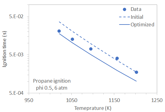
The optimizer identified the top reactions that had the greatest impact on the target. The ratios of optimized to initial rate constants for those reactions are listed in Table 2.7: Reduction in target error after optimization and change in rate constants at 1100K for the reactions optimized along with the level of reduction achieved in the target error. Comparison of the calculated ignition times using the initial and optimized mechanisms to the data are shown in Figure 2.11: Comparison of the initial and optimized propane mechanism with user data for ignition time. Further optimization may be achieved by increasing the number of function evaluations for the optimization methods.
Table 2.7: Reduction in target error after optimization and change in rate constants at 1100K for the reactions optimized
| Target error BEFORE → AFTER optimization = 0.082 → 0.013 | ||
| No. | Reaction | k(optimized/initial) at 1100K |
| 138 | C3H4+OH=C3H3+H2O | 0.69 |
| 145 | C3H5+OH=C3H4+H2O | 0.72 |
| 147 | C3H3+HO2=OH+CO+C2H3 | 0.16 |
| 150 | C3H6+OH=C3H5+H2O | 1.86 |
| 154 | C3H5+HO2=C3H6+O2 | 2.39 |
| 155 | C3H5+HO2=OH+C2H3+CH2O | 7.05 |
| 164 | C3H8+O=I-C3H7+OH | 4.58 |
| 165 | C3H8+O=N-C3H7+OH | 11.59 |
| 166 | C3H8+OH=N-C3H7+H2O | 0.89 |
| 167 | C3H8+OH=I-C3H7+H2O | 0.47 |
Figure 2.11: Comparison of the initial and optimized propane mechanism with user data for ignition time
This tutorial demonstrates the Global Mechanism Optimization capability in Reaction Workbench to optimize a surface kinetics mechanism. The tutorial uses a model for the CVD of silicon nitride in a process that operates at a low pressure of 1.8 Torr, and a high temperature of 1440 C. Modeling of the process using a steady-state PSR model is described in a lesson in the Chemkin Tutorials, "PSR Analysis of Steady-state Thermal CVD" (section 4.1.2). That manual also provides a description of the chemistry set used, in the section, "Silicon Nitride CVD from Silicon Tetrafluoride and Ammonia." The gas phase mechanism includes 17 species and 33 reactions. The surface mechanism contains 6 surface sites, bulk phase Si(D) and N(D), and 6 reactions.
The project file is mechanism_optimization__psr_cvd.ckmop, located in the samples<release_number> directory. Supporting files are located in the mechanism_optimization\PSR_CVD subdirectory. The corresponding Chemkin reactor model setup is the same as that described in the tutorial mentioned previously of the Chemkin Tutorials, except for one modification. The variation in inlet fractions of SiF4 has been modeled here as a Parameter Study and not as Continuations. There are five parameter runs where the mole fraction of SiF4 increases from 0.14 to 0.22.
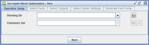
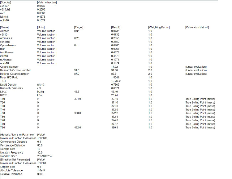
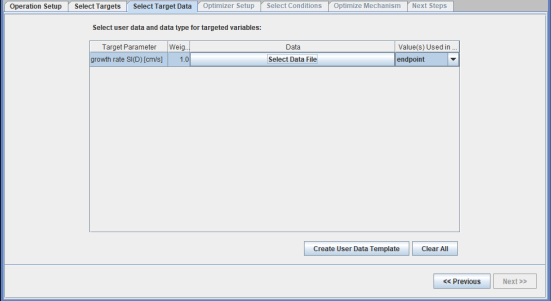
User-provided data are selected as the target for optimization, as shown in Figure 2.12: Operation Setup panel of the Global Mechanism Optimization project for optimizing surface kinetics mechanism . We will optimize the surface mechanism by selecting the check box. In addition, the option to optimize only selected reactions has been selected. Reactions can be selected by clicking the View/Select button, which brings up the panel as shown in Figure 2.13: Pop-up panel to select reactions from the surface mechanism to optimize. Reaction 2 has been selected for optimization in this example. Multiple reactions can be selected if needed. On the next tab of Select Targets, the variable "growth rate SI(D)" has been selected as the optimization target. On the Select Target Data tab, a .csv file containing the data on growth rate of silicon, SI(D), has been imported. A formatted template of the .csv file can first be created by clicking the Create User Data Template button on the same panel. This .csv file contains entries for the parameter study setup from the Chemkin project. Target data are added in the last column of this .csv template file. File Si3N4_deposition_param.csv containing the target data can be found in the working directory. If more than one target is selected, non-unity weights can be specified on this panel, if needed.
Figure 2.12: Operation Setup panel of the Global Mechanism Optimization project for optimizing surface kinetics mechanism
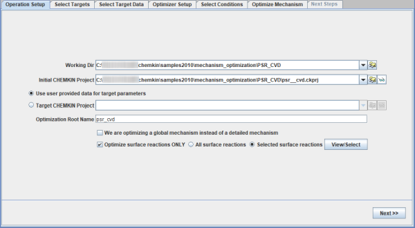
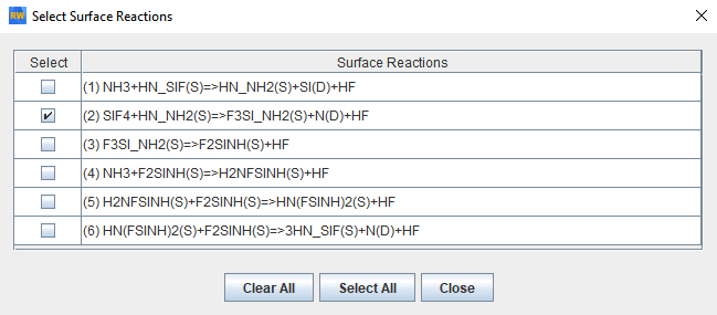
Figure 2.14: Select Target Data tab for creating user data template and importing the target data .csv file
The optimizer setup is the same as that described in Mechanism Optimization for Ignition-delay Times for Propane Autoignition. Function evaluations for global (genetic algorithm) and local (direction set) optimization methods have been restricted to 20 and 10, respectively, for this example. When optimizing a large number of reactions, these evaluations would need to be increased. Using the default number of evaluations of 2000 and 1000 is recommended.
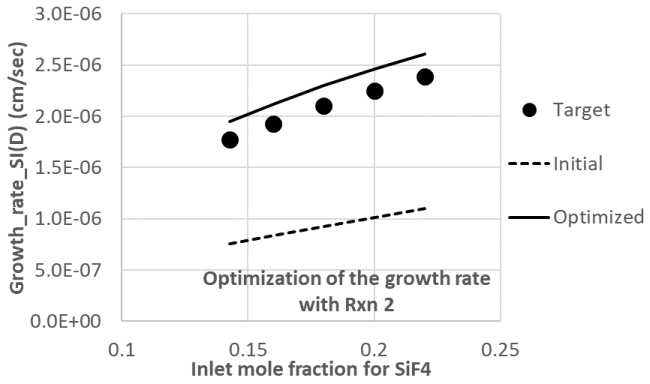
The optimizer attempts to optimize the rate parameters of the selected reaction in the surface mechanism. Note that gas phase reactions are kept as-is when optimizing the surface mechanism and vice versa. An optimized mechanism, with target error reduced by over an order of magnitude from the initial, was generated, as shown by the results on the Optimize Mechanism tab (Figure 2.15: Optimize Mechanism panel of the Global Mechanism Optimization project for optimizing surface kinetics mechanism). The optimized mechanism captures the impact of increasing the inlet concentration of SiF4 on the deposition growth rate of silicon nitride, as shown in Figure 2.16: Comparison of the initial and optimized surface mechanism with the user data for silicon nitride deposition.
The optimization is not fully completed with the reduced number of function evaluations for global (genetic algorithm) and local (direction set) optimization methods, of 20 and 10, respectively. Further optimization can be made by increasing these numbers of function evaluations. Even with the current settings, however, substantial optimization has been achieved.
Figure 2.15: Optimize Mechanism panel of the Global Mechanism Optimization project for optimizing surface kinetics mechanism
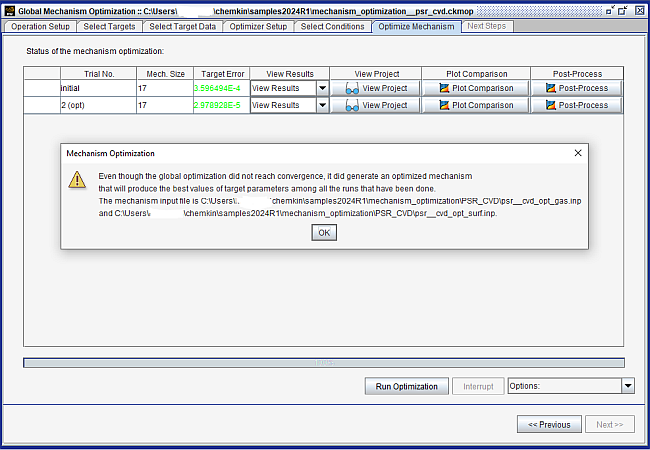
Figure 2.16: Comparison of the initial and optimized surface mechanism with the user data for silicon nitride deposition