


This section provides a guideline to set up generic internal combustion engine cases using Ansys Forte. The geometric setup of such engine cases includes not only the combustion chamber, but also the intake and exhaust ports and the valves within. Valve motion is simulated to account for the realistic gas exchange process in the engine. This guideline emphasizes the considerations you must pay attention to when working on such cases.
This section is arranged in the following parts:
General notes on the use of Ansys Forte and configuring it for your use:
The surface mesh file should have the piston at TDC.
The valves should be closed with a very small gap, but not coincident.
This section introduces how the surface mesh geometry should be read in and what you need to do to facilitate the subsequent setup stages. Specifically:
Selecting the Source of Surface Meshes introduces the best practice of importing a surface mesh into Forte.
Splitting the Geometry introduces how to split the surface mesh into different parts to help set up an engine simulation case.
Normals introduces the requirements of surface normal vectors and how to fix the inverted normals.
The best surface mesh data include surface topology information. The Fluent mesh format and CGNS format include topological information about the surface and are good choices for import.
Whenever possible, STL files should be a last choice as a source of surface mesh data. STL files lack surface topology information. As different programs may infer different topologies from the same source file, there is no way to reliably confirm or test whether an STL is, for example, watertight.
Currently, the best alternatives to STL files supported by Ansys Forte are Fluent mesh format and CGNS format. Both of these formats encode topological information about the surface.
A recommended procedure for generating a surface mesh for importing to Forte is:
Create a "Mesh" object in Ansys Workbench and import your geometry, then launch the mesher.
Configure the mesher to CFD, Fluent, and specify these options:
Defaults:
Physics Preference = CFD
Solver Preference = Fluent
Sizing:
Transition = Slow
Defeaturing:
Automatic Mesh Based Defeaturing = ON
Other settings may also be adjusted for good results.
Generate just the surface mesh by right-clicking the Mesh object > Preview > Surface mesh.
Go to File > Export and save the .mesh file.
In Ansys Forte, import the surface mesh using the From Fluent mesh import option, and select meters as the units.
Reverse the normals for the imported surface—everything should go from dull to shiny.
If the geometry comes into Forte as one complete surface, you will first
need to split it into major components. This can usually be accomplished with a
simple application of the Split Mesh  utility in the Geometry workflow tree,
using the default Feature Angle.
utility in the Geometry workflow tree,
using the default Feature Angle.
If you end up with some small pieces, try to collect those and merge them into the bigger pieces, using the Merge Meshes
 utility.
If you need to split surfaces further, consider using the Cut by Plane option or adjusting the Feature Angle that was used for the Split Mesh utility.
Ultimately, you want to end up with the following surfaces that are separated and free of holes:
Individual valves
Exhaust port wall
Intake port wall
Cylinder head
Cylinder liner
Piston surface (usually including bowl)
Inlet boundary
Outlet boundary
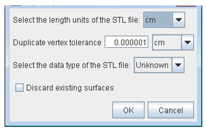
It is easiest if the separate boundaries, such as ports, valves, etc., are written as separate parts in the surface mesh file or as separate surface mesh files all together. You can select multiple surface mesh files to read into Ansys Forte. (The surface mesh must be watertight.) Once again, the geometry should be in units of cm in Forte. If the geometry is not in cm, specify the unit used for the geometry and Forte will convert the geometry to cm units upon reading it into the user interface.
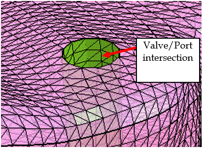
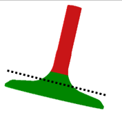
The valve stems should be cut and flush at the location where they meet the port (at the end of the valve stem/port connection).
Figure 4.3: The valve (green region), the port (pink region), and the donut surface around the intersection of the two
Note: If the crevice volume is included in the geometry, this volume must be resolved sufficiently using surface refinement such that there is at least one layer of cells between the two walls of the crevice gap. However, resolving the crevice gap using tiny cells will increase the cell count of the mesh and potentially affect solution speed. Therefore, it is desirable to not include the crevice region in the geometry unless it is absolutely necessary. For more detailed information, refer to Modeling the Crevice.
In the surface mesh geometry, the normals must all be consistent. The normals should all point to the solid region, so for the valves, the normal should point to the center of the valve.
If the normals for some triangles are not consistent, the geometry is not considered to be watertight and these triangles will be highlighted with a red outline.
To separate these inverted triangles, go to the Geometry workflow tree and select the surface that contains the inverted triangles. Split Mesh
and select the Feature Angle
option. On the Feature Angle dialog, specify a Feature
Angle of 175 as shown in the figure below. 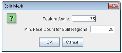
This will split off all inverted triangles, and you can then use the Inverse Normals tool
 to correct the normal.
 Note that the geometry will not be watertight at this point since the triangles are not considered to share vertices. To fix this, the final step is to use the Join Meshes
 (not to be confused with the Merge
Meshes ) tool to join all the surfaces back together. At
this point, the red outline of the offending triangles should
disappear.
(not to be confused with the Merge
Meshes ) tool to join all the surfaces back together. At
this point, the red outline of the offending triangles should
disappear.
Note: If you get a mesh-generation failure when validating project settings, an incorrect surface normal is a very likely cause.
This section illustrates the settings needed to use Ansys Forte's Automatic Mesh Generation for the volume mesh.
For a related video that provides an overview of the content covered in these steps, see ANSYS Forte: Mesh Refinement Strategies on the Ansys How To Videos page.
In addition:
Modeling the Crevice provides best practice guidance to model the crevice volume in the combustion chamber of your engine.
Modeling Sector Geometry Using Automatic Mesh Generation provides the best practice guidance if you only need to model a cylindrical sector of the engine combustion chamber, instead of the 360-degree "full sector" of the engine.
Multi-Cylinder Simulations provides a link to the tutorial to perform multi-cylinder instead of single-cylinder engine simulations.
The Material Point marks the location where Forte will generate the volume mesh for the fluid domain, that is, marks what is considered inside and outside of the geometry where the surfaces mark the boundaries of the fluid domain.
Select a point that will always be inside the combustion chamber cylinder during the engine cycle. Usually this means a location just below the cylinder head surface, at the cylinder axis, above the highest point of the piston bowl (that is, at the piston's Top-Dead-Center, or "TDC"). Be sure the material point is not placed in-line with any of the valves to avoid the valve motion sending the material point outside the fluid domain.
The Global Mesh Size provides the base mesh size of Ansys Forte's Cartesian Octree meshing solver. The Global Mesh Size is used everywhere a mesh refinement is not specified. In Ansys Forte, a global mesh size of 2–2.5 mm is suggested. Mesh size and simulation turn-around time requirements are often competing forces, therefore one must balance these two.
A recommended global mesh size for generic engine cases is 2 mm. But for large-bore diesel engines, it may be acceptable to use 3 mm for the flow portion of the cycle, while for a smaller-bore gasoline engine 1.5 mm may be more appropriate. Then, use the measures in Mesh Refinement to refine the mesh based on the global mesh size.
Ansys Forte uses automatic meshing with Octree-structured Cartesian cells to generate the volume mesh for the simulation domain. The actual meshing is done automatically on the fly by the Forte solver. When setting up the project, it is recommended to specify mesh refinement controls to resolve certain shapes and features of the geometry and to apply certain models.
Mesh Refinements are used to resolve both surfaces and regions within the simulation domain. All types of mesh refinements are added as fractions of global mesh size, which would be 1/2, 1/4, 1/8, 1/16, 1/32, and 1/64.
In engine simulations, note that refinements should be added to sufficiently resolve all crevices in the engine geometry, that is, small physical gaps between the piston edge and the cylinder walls, otherwise robustness may be affected. (See Modeling the Crevice.)
Each of the mesh-size controls can be specified as static (Always active) or dynamic (active only During specified time or crank-angle intervals). The dynamic mesh-size controls are helpful in controlling computational cost by refining meshes only when needed. For example, refinement in the squish region near a moving piston boundary may only be necessary when the piston is near its TDC position. For simulation of a full engine cycle, this may mean setting two controls for the two Crank Angle ("CA") intervals (for example, 350 to 370 CA degrees, 710 to 730 CA degrees) during the cycle of a 4-stroke engine while the combustion physics in the squish region is most active.
Ansys Forte has several refinement types that are useful for resolving the simulation domain. They fall in two main categories: (1) surface refinement, and (2) volume refinement. Volume refinement is further divided into two categories: (2a) fixed volume refinement, and (2b) Solution Adaptive Meshing (SAM). Surface refinement should be used in every case. SAM with limited fixed volume refinements is recommended for volumes.
Surface Refinements:
Applied to surfaces to refine the volume meshes nearby. In engine cases, mesh refinements are needed for wall boundaries, open boundaries, valves, as well as surfaces with complex geometries and small features (such as spark plug, crevice, and so on).
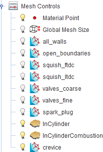
Figure 4.4: Suggested refinements for typical engine cases shows the suggested refinements to be used for most engine cases. Details of each refinement are given.
all_walls: Surface refinement applied to all wall boundaries as a base setting. Typically, ½ refinement is used (Active = Always).
open_boundaries: Surface refinement applied to the inlets and outlets of the domain. Typically, ½ refinement is used and the number of layers to extend is specified as 2 (Active = Always).
squish_ftdc and squish_ltdc: Surface refinement applied to the head, piston, and liner surfaces, which form the enclosed squish region. This refinement is active only for the TDC events. Typically, ¼ refinement must be added such that the TDC clearance height is resolved (Active = During).
valves: Surface refinement applied to the intake and exhaust valves. Typically, ¼ refinement is required on the valve. The valve may be split into two parts, stem and face, to save a mesh count with deeper refinement applied only to the face near the seating area (See Valves for more details). If more refinement is desired near the valve seating area, ¼ refinement can be applied to the head or port regions near the valve.
crevice: If a crevice volume is included between the piston edge and the liner wall, this area should be resolved sufficiently using surface refinements such that there are 2 cells across the crevice gap. Typically, 1/8 refinement is needed with multiple cell layers extended from the surface to fill the crevice gap. To reduce the mesh count, the piston or liner surface can be split to apply deeper refinement only to surfaces that form the crevice (Active = Always). (See Modeling the Crevice for more details).
spark_plug_surface: For engine cases with spark plugs, surface refinement is needed to resolve the spark plug's geometric structure properly. Typically, 1/8 refinement is used to sufficiently resolve the geometry and the spark gap, but this will depend on the specific spark plug geometry. If there is any gap other than the spark gap (discussed below), it should have at least one layer of fluid cells. If there is any thin wall in the spark plug geometry, local mesh refinement should make sure that the thin wall does not run through any fluid cells. (Active = Always).
spark_plug_region: In addition to the surface refinement, you need to set Point Refinement centered at the spark plug to provide reasonable resolution for the spark ignition and early-stage flame propagation models. The point refinement radius is typically specified such that 6 to 10 layers will resolve the region around the spark plug and the resulting flame front. Sometimes two-to-three point refinements with different spherical radii and refinement levels are needed to balance between the need for refinement and computational cost. Such refinements should be active only within a short duration during the spark ignition and early-stage flame propagation (Active = During).
Mesh resolution in the spark gap region needs particular attention. The combination of the above-mentioned surface refinement and point refinement should result in about 3 layers of cells across the spark gap if using the DPIK spark model, and about 5 layers of cells across the spark gap if using the ACT spark model (see Spark Model for details about these two models) during the spark ignition.
Note: It is recommended to use a SAM refinement to capture the later-stage flame propagation. Refer to SAM Settings for Flame Propagation for details.
Injector and glow plug: Surface refinement applied to the injector tip. Typically, ¼ refinement is used to sufficiently resolve the geometry and the number of layers to extend refinement is typically 2 (Active = Always).
Feature refinement: This type of refinement can be specified on single or multiple surfaces. A feature angle is specified to identify features on surfaces (smaller angle = greater feature refinement). A radius that is applied to each identified location is also specified. This option is useful when refining oddly shaped geometry.
Volume Refinements:
Volume refinement is important to achieve mesh-independent results. SAM is recommended as it does not require prior knowledge of the solution field and it saves time and mesh count while producing accurate results. In addition to SAM, some fixed-volume refinement is recommended for certain cases.
(2a) SAM controls:
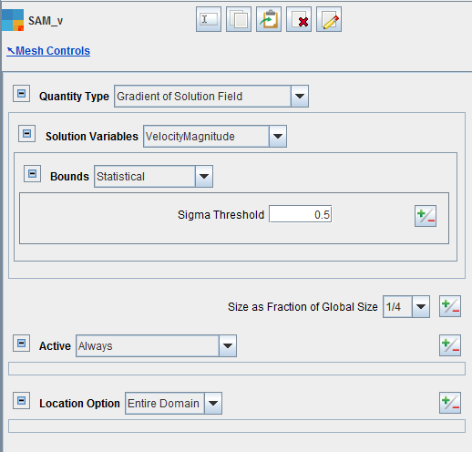
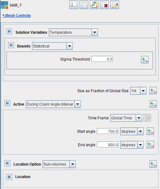
SAM should be used to resolve the flow field and chemically reactive zones. Recommended options are using velocity gradients and temperature gradients with statistical sigma threshold of 0.5, and ¼ refinement (for global mesh size ~2 mm). Velocity control should be active always and be applied to the entire domain (Figure 4.5: SAM control for resolving flow fields). Temperature control can be limited to the cylinder region and be activated prior to TDC for the combustion duration, as shown in Figure 4.6: SAM control for resolving chemically reactive regions.
Additional SAM controls should be used for accurately capturing the flame front and spray vaporization. These are described in SAM Settings for Flame Propagation and SAM Settings for Spray Vaporization, respectively. Additional SAM controls on species such as CO or soot precursors (like acetylene and pyrene) may be used to better resolve emissions but they are not necessary.
(2b) Fixed volume refinements:
In certain situations, fixed volume refinement should be used to provide some level of initial refinement in the regions where intensive physical and chemical processes (for example, combustion and sprays) occur. These fixed refinements provide a good base mesh and help to achieve high fidelity results when used together with SAM.
Point Refinement:
Point refinement is typically used to refine the regions around the spark plug. See the discussion of spark_plug_region above.
Secondary Volume:
This option is useful when the engine has very large intake/exhaust manifolds and must use a very large global mesh size (4 mm or 6 mm). In this case, you can set up a Secondary Volume for the combustion chamber so that a smaller mesh size can be used within. Under the Geometry node, Sub-Volumes can be defined by selecting geometry to encapsulate a specific region in the simulation domain. In our example, this region is the in-cylinder volume enclosed by the liner, piston, and head surfaces. Under the Mesh Controls, the Secondary Volume option can be used to refine meshes in a sub-volume. The refinement level for the in-cylinder region should be set to ½ or ¼ to achieve a cell size around 2 mm in the combustion chamber and set to Always Active.
Caution: We recommend using this option only when the global mesh size has to be very large. Otherwise, use of this option could significantly increase the overall mesh size and computational time.
Line Refinement:
One very useful case for this type of refinement is discussed in Modeling Sector Geometry Using Automatic Mesh Generation. There are two additional, but uncommon, use cases: (1) The end points of a line and a radius could be specified to define a cylinder where all locations inside the cylinder are refined to the specified refinement level. (2) Line refinement could be used to resolve near-nozzle regions during spray duration. Point refinement can be used instead of line refinement depending on the geometry. Although, the best way to refine meshes around sprays is to use SAM (See SAM Settings for Spray Vaporization).
While it is recommended not to modeling long narrow crevices (unless there is some engineering reason to do so) due to the computational overhead, such crevices may be included if necessary. The best approach to model the crevice is to do the following:
Have a separate surface for the bottom of the crevice.
Split the piston so the side of the piston becomes a separate surface.
Apply 1/8 or 1/16 refinement to the crevice bottom surface and the piston-side surface. The crevice thickness will determine the refinement level to be used, but 1/8 or 1/16 is typically used to resolve the thickness.
If possible, modify the geometry such that the crevice thickness can be greater while capturing the same volume, to avoid many highly refined cells.
Forte allows cylindrical sector geometry (with periodic boundary conditions) to be meshed using automatic mesh generation. This is complementary to the body-fitted sector mesh feature described in DI Diesel Engine Case (Typically, Sector Mesh). Since the automatic mesh generation in Forte uses the Cartesian mesh with immersed boundary method, it is necessary to make sure that the background Cartesian mesh cells near the geometry boundaries are sufficiently refined, especially near the axis of the sector.
To avoid display artifacts in post-processing, a Line Refinement can be applied along the sector axis. The following are recommended settings for this line refinement:
End Points: This line refinement should cover the full length of the axis when the piston is at the Bottom-Dead-Center ("BDC") position. The end points can be set to (X=0, Y=0, Z1) and (X=0, Y=0, Z2), in which Z1 is the Z-coordinate of the top end of the axis on the cylinder head, and Z2 equals the Z-coordinate of the piston center at the TDC position minus engine stroke (assuming the piston moves towards the negative Z direction from TDC to BDC).
Radius of Application: The radius should be larger than half of the global mesh size. Recommended practice is to set the radius equal to the global mesh size.
Size as Fraction of Global Size: The cell size of this refinement should be equal or smaller than the cell sizes from other refinements. The goal is to maintain uniform cell size within the range of this line refinement.
Active: This refinement should be set to be Always active.
Note: Best practices for multi-cylinder simulations are described in Multi-Cylinder Four-Stroke Engine Simulation in the Ansys Forte Tutorials.
This section introduces the best practice in setting up physical models for the engine simulations. Specifically:
Turbulence Model introduces the recommended settings for turbulence model. The flow processes in engines are generally turbulent.
Flame Speed Model for SI Engine Simulations introduces the recommended settings for the flame speed model. This model is used in engines that have flame propagation, which are usually spark-ignition (SI) engines.
Spray Model introduces the recommended settings for the spray model. Spray model is required in engines using liquid fuels and need to simulate the fuel-air mixing processes.
Spark Model introduces the recommended settings for the spark model, which is used in SI engines.
Soot Model introduces the recommended settings for the soot model, which is needed when soot emissions are to be predicted.
In modeling turbulent flows in internal combustion engines, the Reynolds-Averaged-Navier-Stokes approach is most efficient. It simulates the ensemble average of turbulent flow and transport processes. The default option, RNG k-ε model, is recommended for most of the engine flow and combustion problems. In general, there is no need to adjust the default model parameters.
The Large-eddy simulation (LES) approach is intended to simulate individual flow realizations rather than the ensemble average. It is useful when simulating cycle-to-cycle variations of flows and combustion outcomes in engines. The LES Smagorinsky model with its default model parameters is recommended, due to its numerical stability in cases where complex engine geometry is considered. When the LES approach is used, turning on the option of using Central Difference for Momentum Convection is recommended, due to its better resolution in solving the large-scale momentum transport.
In general, LES requires finer mesh resolution than RANS to better resolve the turbulent transport processes.
The Flame Speed Model under the Chemistry/Materials node can be used to control the flame propagation process for a spark-ignited engine simulation. Using the Table Library option for the flame speed model is recommended.
Typical values for the parameters that control flame speeds are shown in Figure 4.7: Turbulent flame-speed input parameters.
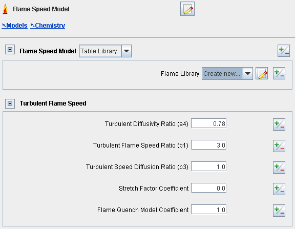
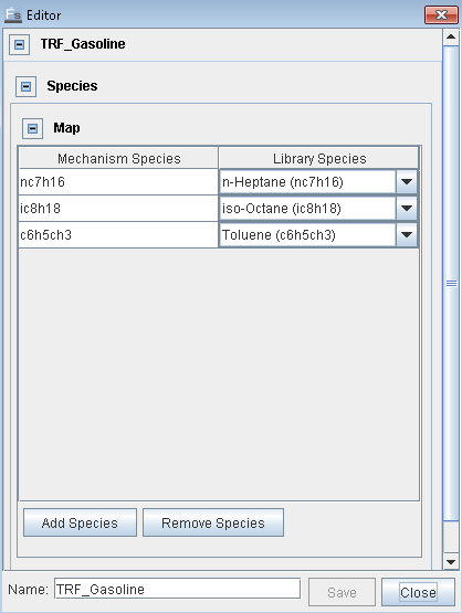
The turbulent flame speed is a function of the laminar flame speed. The Table Library model contains Chemkin-based laminar flame speeds and computes flame speeds for the multi-component fuel on the fly. It captures the influence of fuel composition, pressure, temperature, AFR, and EGR on the laminar flame speed. A Flame Library should be created that includes fuel components when premixed or direct-injection fuel surrogate are used in the chemistry. An example flame library for a TRF gasoline is shown in Figure 4.8: Example of a Flame Library for a TRF gasoline.
The Turbulent Flame-Speed Ratio (b1) and the Stretch Factor Coefficient are the two inputs that may require adjustment to match the pressure trace in a spark-ignition engine. See the tooltips of these parameters and General Formulation and Turbulent Flame Speeds in the Ansys Forte Theory Manual for more details on these inputs. Since the model formulation for the stretch factor is very sensitive to its input parameters, including laminar flame speed, laminar flame thickness, and turbulence parameters, the stretch factor may show strong fluctuation under strong turbulence and low laminar flame speed conditions. Therefore, it is recommended to keep the default setting of 0 for the stretch factor coefficient, and adjust only b1. In the turbulent flame-speed correlation used by Forte, b1 is closed using experimental data and thus can be adjusted for model calibration. A larger b1 will result in higher turbulent flame speeds and faster flame propagation, and it has an impact throughout the flame propagation process. If unable to match the pressure curve during flame propagation by adjusting b1, the Flame Development Coefficient (FDC), which is another parameter available on the Spark Ignition editor panel, can be adjusted to improve flame propagation prediction. A larger FDC can result in faster growth of the flame from ignition kernel flame stage to fully-developed turbulent flame, which in turn leads to faster burn rate. FDC typically has larger impact on the early stage of flame propagation than the later stage. For the other settings, default values are appropriate for most cases.
For chemistry in the flame-front region, the default Equilibrium option will be sufficient if flame temperatures will be high. If flame temperatures might be on the order of 1500 K due to operating conditions that result in locally fuel-rich or high EGR conditions, the Stirred Reactor model is recommended, especially if soot must be calculated.
For the Unburned Calculation Method used to compute unburned conditions, use the Volume Search with Variable Radius option, which is the default option since Forte 2024 R2. Do not use the other options.
Do not enable the Use Legacy G-Convection Formulation or the Use Legacy Method for Flame Front and High-Temperature Front Synchronization options.
In Ansys Forte, flame propagation is simulated by the G-equation model. For achieving accurate and mesh-insensitive flame propagation, it is recommended to use SAM Controls with Absolute Range Bounds and G for Solution Variables as shown in Figure 4.9: SAM settings for flame propagation. This setting will help refine the region around the flame front as defined by G=0. This refinement should be activated typically at spark ignition and typically for 60 degrees longer until combustion is complete. The recommended cell size for accurately capturing the flame front is no larger than 0.6 mm. On the other hand, the G-equation model does not require cells in the flame front zone to be deeply refined. Therefore, if the global mesh size is about 2 mm, the best practice is to use ¼ refinement in the G-based SAM for the whole flame propagation process.
During the ignition kernel stage, the spark ignition zone needs sufficient mesh resolution using fixed refinement (see spark_plug_region in Mesh Refinement). Alternatively, you can consider applying a second SAM-G refinement with 1/8 refinement and apply it only for a short duration, for example, 10 CA degrees after spark timing.
In the G-equation model, the non-reacting scalar G is defined at each mesh vertex for the purpose of marking the mean flame front location. The G value at a vertex is tracked as the signed normal distance from the vertex to the nearest flame front surface. G < 0 in the unburned zone, G > 0 in the burned zone, and the G=0 iso-surface marks the flame front location. Since Forte uses the CGS unit system, the default unit for G is cm, although G is handled as a dimensionless quantity internally and it involves no unit conversion. In the example shown in Figure 4.9: SAM settings for flame propagation, the range of [−0.3, 0.3] means that the SAM refinement is applied within a band surrounding the flame front. The band widths on the unburned side and burned side are 0.3 cm and 0.3 cm, respectively.
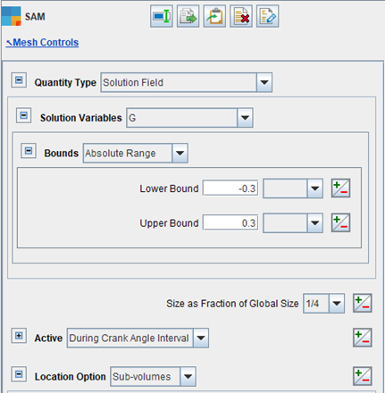
Tip: It is acceptable to let the SAM controls with G for Solution Varibles as indicated in Figure 4.9: SAM settings for flame propagation to be Always Active during an engine cycle. When the spark ignition or G-equation model is inactive, the default G value is -1.0e+6, hence no vertices will have G values within the specified range (-0.3 to 0.3), so this SAM control is essentially ignored.
In addition, it may be productive to use additional SAM controls with gradients of either/both temperature and of CO. Using temperature/CO control can be helpful for high compression conditions where there could be a possibility of autoignition or reactivity ahead of the flame front. It is recommended to use statistical bounds with a Sigma Threshold of 0.5 to 0.75 for temperature. Using a smaller sigma value results in more refinement. This refinement should be activated at or slightly prior to spark timing.
In general, most of the defaults can be used for the spray model for the injector. The default Adaptive Collision Mesh model for droplet collision is suggested for better computational speed. For Solid Cone Injectors, a Droplet Density option with a value of 1 is recommended. When nozzle dimensions are available, using the Nozzle Flow Model may provide better spray initialization at the nozzle exit. However, for gasoline sprays using Rosin-Rammler or Log-Normal droplet size distribution, explicitly specifying the Discharge Coefficient should provide better representation of the injector exit. The discharge coefficient for multi-bore high pressure injectors can be as low as 0.5, which is lower than that for most diesel injectors.
For diesel fuel, specifying Uniform Size for the droplet size distribution is suggested. For gasoline sprays, Rosin-Rammler Distribution is more commonly used than Log-Normal Distribution. The Initial Sauter Mean Diameter should be specified. For most gasoline cases, this is typically between 10–30 micron. The actual droplet distribution is subject to an upper limit, which is the (nozzle diameter * Cd0.5).
For Solid Cone Breakup Model Settings, time constants for the KH Model (primary breakup) can be adjusted within the range suggested in the tool tip. The check box to Impose SMR Conservation in KH Breakup should be left unchecked for most conditions. However, it can be turned on for certain conditions such as low-load low-temperature combustion diesel engines, for improving the pressure curve and emissions predictions.
The RT Model for secondary breakup is important for most conditions. The RT Distance Constant can be adjusted to improve the prediction of both spray penetration and combustion. A lower value of the RT distance constant, such as 0.2, will activate the secondary breakup model closer to the nozzle. This may be important for gasoline atomizers where spray breakup occurs very close to nozzle. For most diesel engines, the RT distance constant typically varies within 40% of the suggested default value of 1.9. Refer to Table 4.1: Parameters providing secondary impacts on engine behavior for the typical qualitative impact on the predicted engine behavior.
When creating nozzles, first create one nozzle and specify all its settings,
and then use the Copy![]() and Paste
and Paste![]() buttons at the top of appropriate Editor panels repeatedly
to create the remaining nozzles, modifying the copied settings as needed. This
saves time and only one parameter must be adjusted to change the
orientation.
buttons at the top of appropriate Editor panels repeatedly
to create the remaining nozzles, modifying the copied settings as needed. This
saves time and only one parameter must be adjusted to change the
orientation.

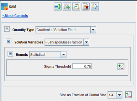
Spray vaporization can be quite sensitive to cell size. Therefore, it is advisable to use finer mesh to accurately account for vapor distribution and mixing. As shown in Figure 4.11: SAM settings for spray vaporization, SAM controls should use the gradient of solution field on variable FuelVaporMassFraction with the statistical sigma threshold between 0.5 to 0.75. Smaller sigma value results in more refinement. Recommended cell size for accurately capturing the vaporization is no larger than 0.5 mm. For example, if the global mesh size is around 2 mm, the refinement level can be set to ¼.
For the Discrete Particle Ignition Kernel (DPIK) Spark Model, the Duration of the spark is typically about 10 CA degrees, the Energy Release Rate is about 30 J/sec, the Energy Transfer Efficiency is 0.5, and the Initial Kernel Radius is about 0.5 mm. The initial kernel radius should be sufficiently small to fit in the spark gap, but remember that the spark gap should also be sufficiently mesh-refined so that at least 3 layers of cells can fit inside the spark gap.
For the Arc Channel Tracking (ACT) Spark Model, if the Electric Circuit Discharge Model is used to compute the spark energy discharge rate, the default values for the electric circuit configuration parameters should be a good starting point. This model requires the surface geometry to contain the anode and cathode structure of the spark plug because the motion of the flame particles on the two ends of the arch channel will be constrained to slide along the anode and cathode walls. During ignition, the spark gap region should be sufficiently refined so that at least 5 layers of cells can fit inside the spark gap. The particles in the ACT model are driven by the mean flow velocity (subject to other constraints), so it requires the flow field in the spark gap region to be well resolved.
Ansys Forte has three options for modeling soot:
The Two-Step Soot Model: The two-step soot model in Forte is a model where only acetylene (C2H2) is the precursor to soot formation. Several values are available for adjusting the soot formation and oxidation. This option should be selected if acetylene is the only precursor for soot. Note that the gas-phase chemistry mechanism must contain soot as a species when this soot model option is used.
Pseudo-gas Soot Model: The pseudo-gas soot model was developed by Ansys and is included with the gas-phase chemistry set. A gasoline and diesel surrogate and mechanism are provided with the Forte installation. If you are using the pseudo–gas-phase soot model, the Soot Model option in Forte should not be selected since all soot-related chemistry is included in the gas-phase chemistry file.
Method of Moments: The most detailed option for modeling soot is particle tracking. Forte will predict the average particle size and number density for every cell in the computation. To use this option, choose the Method of Moments. There are two mechanisms for particle tracking included with Forte, one for gasoline and one for diesel fuel. The Method of Moments option requires specifying the soot surface chemistry mechanism.
This section highlights a few best practices on the boundary conditions used in typical engine simulations. Specifically:
Boundary Profiles discusses the use of "profiles" to specify time-varying boundary conditions.
Valves provides a tip to split the valve surface mesh to facilitate mesh refinement settings.
Valve Angles provides guidance on setting the valve tilt angles for the purpose of specifying the direction of valve motion.
Valve Lift is about the usage of profiles to set up the magnitude of valve motion.
Movement Type discusses the boundary condition settings for piston, valves, and sliding interfaces. The valves are discussed in detail here.
Inlet Boundary introduces the usage of inlet boundary conditions in engine simulations.
Outlet Boundary introduces the usage of outlet boundary conditions in engine simulations.
In Ansys Forte, it is very easy to use profiles for time-varying boundary conditions, for example, valve lifts. When specifying time-varying profiles for engine cases in Forte, the profile should go from 0 to 720 CA for a four-stroke engine and from 0 to 360 CA for a two-stroke engine. By specifying the profile in this manner, it is easy to then run multicycle engine simulations. Profiles can be copied from Excel and pasted in the Profile Editor.
In this section, the setup of the intake valve is described. The same setup and procedure would be used for the exhaust valves. It is recommended that you set up one valve, then Copy and Paste it to create the other valves.
In the setup as shown in Figure 4.12: Valve stem split off from the valve face, the valve stem has been split off from the valve face. This has been done to improve the speed in the calculation where Forte determines if the valve is open or closed, that is, the specified gap between the valve and valve seat has been obtained. Splitting off the valve face from the stem is not required, but it may improve simulation time since the mesh refinement for the valve opening gap is only applied to the valve face and not the entire valve (see also valves in Mesh Refinement).
The easiest way to specify valve tilt angles (orientation) is to use spherical coordinate systems. This will be explained using one example shown in Figure 4.13: Valve tilt angles. In this example, the engine geometry is oriented such that the engine valves are tilted in the X-Z plane. When looking from the negative Y direction, the intake valves are on the right and the exhaust valves are on the left. In this configuration, the spherical coordinate system for each valve requires two angular inputs, θ and φ, where θ is the valve angle to be specified and φ can be left as zero. The valve angles will be:
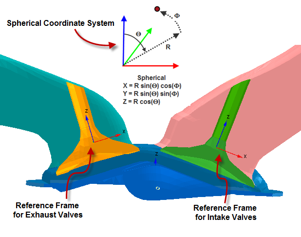
Intake Valve Angle(θ) = 180 + valve_angle, for example, if the valves are canted 13 degrees, then the resulting angle would be 193 degrees.
Exhaust Valve Angle(θ) = 180−valve_angle, for example, if the valves are canted 12.6 degrees, then the resulting angle would be 167.4 degrees.
For each valve, copy and paste its lift profile into the profile editor. Make sure the profile goes from 0 to 720 degrees for a four-stroke engine and also be sure the units for the profile are correct.
In boundary conditions where Wall Motion is activated, there are three options for the Movement Type:
Moving Surface: Used for the piston.
Valve: As the name indicates, this is used for valves.
Sliding Interface: Used in ported engine cases where the piston covers/uncovers port openings to the cylinder.
For the Valve movement type, the valve seat and the surface it contacts must be specified. The valve seat is the stationary portion that may be a part of the head or intake/exhaust port surface and the surface it contacts is the valve itself.
In this case, some portions of the intake port (similarly for the exhaust port) have been split off and labeled as the "seat". This splitting is not a requirement, but has been done in this case to help with the calculation speed of the valve opening/closing events (see Notes in Valves). The splitting is accomplished with a cut plane in the Geometry tree.
Select both the "seat" portion and the "valve" from the list by holding down the Ctrl key and clicking with the left mouse button to multi-select.
Now that the Valve movement type surfaces have been selected, you must specify the Valve Motion Activation Threshold, that is, the minimum gap before the valve is considered open or closed. It is suggested to start with a 0.5 mm gap in the first simulation. The other required input is the Approximate Cells in the Gap at Minimum Lift and this should be 2.
You can use a smaller gap if you are not satisfied with the results. If high accuracy of valve timing is needed, you can consider setting the Valve Motion Activation Threshold to 0.2 mm and setting Approximate Cells in the Gap at Minimum Lift to 1.5.
The ratio of these two parameters determines the smallest cell size needed in the valve gap at minimum lift. For example, if the activation threshold is 0.2 mm and the number of cell layers in the gap at minimum lift is 1.5, the cells in the gap need to be smaller than 0.2 mm /1.5 = 0.133 mm. In this case, if the global cell size is 2 mm, 1/16 refinement (0.125 mm cell) is needed in the valve gap region at minimum valve lift. Note that Forte automatically refines the valve gap such that the specified number of cell layers can fit in the gap, so no special refinements are required for resolving the gap.
In engine simulations, there are typically two use cases for inlet boundaries:
Inlet boundary for the intake manifold
This type of inlet boundary is typically set at a certain cross-section of the engine's intake manifold to introduce air or fuel-air mixture from upstream. Usually, the pressure at such location is known or measured. Therefore, it is recommended to specify Total Pressure or Static Pressure at the inlet. Specifying Total Pressure is preferred, because it can suppress inhomogeneity of the flow rate and flow re-circulation on the boundary.
For the Temperature Option, if measured data or good estimation is available, the Total Temperature or Static Temperature option can be used to specify constant or time-varying boundary temperature. The Assume Isentropic option can also be used for this use case, but the initial pressure and temperature in the neighboring intake manifold region must be reasonable because these initial condition parameters are used as a reference state in the isentropic assumption.
A Velocity or Mass Flow Rate inlet is not recommended for this use case.
If this is a Spark-Ignition (SI) engine and premixed fuel-air mixture is introduced into the intake port, pay attention to the Composition of the mixture in this boundary condition, as it affects the global equivalence ratio in the engine.
Inlet boundary for high-pressure injector
This use case is for simulating gaseous fuel or air injection in the engine. Such gas injectors can be mounted either inside the cylinder or in the intake system. Typically, there is a large pressure drop across such an inlet. The pressure drop covers a wide range in various engine applications, and it can vary from 10 bar to 100 bar. There are two ways of setting it:
Set the inlet boundary as the exit of the injector nozzle. In this case, the inlet boundary is constantly exposed to the downstream chamber. In this configuration, it is recommended to specify the Mass Flow Rate or Velocity of the injection. Mass Flow Rate is preferred since Velocity is hard to measure directly. A time-varying profile for the mass flow rate or velocity is often needed to simulate the transient effects. Pressure inlet cannot be used in this configuration because it is hard to prescribe boundary pressure values to block the inlet when the injection is not active.
Both the Mass Flow Rate and Velocity options require you to specify the Inflow Mixture Density Option. It is recommended to specify the Pressure (which will be converted into density) or specify the Density directly to define the inflow condition inside the injector. Both total and static quantities are acceptable. Avoid using the Assuming Zero Pressure Gradient option because this assumption is invalid at the exit of a gas injector, and it could cause spurious large velocities near the inlet.
Set the inlet boundary somewhere upstream of the injector nozzle, so that the injector's moving pintle (or needle) is included in the surface geometry. In this case, it is recommended to define the inlet boundary as a Pressure inlet. You can specify constant or time-varying Total Pressure or Static Pressure to match the reservoir condition inside the injector, which is often known for the injector.
In both cases, for the Temperature Option, you should specify the temperature directly to match the reservoir condition inside the injector. Avoid using the Assume Isentropic option.
In engine simulations, there are unique regions that must be initialized with different conditions, that is, the intake, exhaust, and the cylinder. In Ansys Forte, there is always a Default Initialization which will apply to the entire geometry unless other initial conditions are created to "override" the default condition.
To add a new Initial Condition, right-click Initial Conditions and select New Secondary Region from Material Point. You will need to add a total of two secondary regions, one for the intake, and one for the exhaust. The default initialization will be applied to the cylinder, which is the region not marked by either the intake or the exhaust secondary regions.
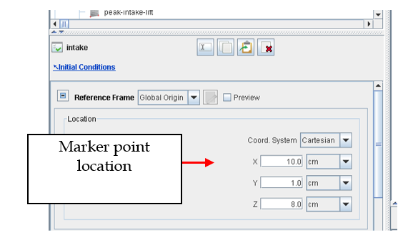
In each new Secondary Region, a material point must be specified to mark it as a unique region, so in this case there would be a material point for the intake and another material point for the exhaust region. The location of these material points does not need to be exact, but they must be completely inside the port (region). Figure 4.14: Indicating the material point location for a region shows where to input the location information for the material points in the initial condition panel of a secondary region.
In Forte, an initialization order is needed to help define region ID values on cells and vertices at the interfaces of different regions, especially when the regions are connected by flow. As a general guideline, the orders should be specified in the direction of flow, so they would be:
Intake: Initialization order = 1
Default Initialization: Initialization order = 2
Exhaust: Initialization order = 3
If you are running a sector mesh, or a combustion/expansion stroke only and the valves are not included, you will only have one initialization (the default) and the initialization order for that region would equal 1.
Time Step
Ansys Forte uses an adaptive time stepping approach where a value for the maximum time-step size is specified. The maximum time-step size in Forte can be a constant value or a profile, that is, a function of time or crank angle. The following are suggestions for maximum time-step size:
Sector Mesh Cases: 8E-06 s during compression, 5E-06 s during fuel injection, combustion and expansion (Note, it may be possible to increase the time-step size back to 8E-06 s late in the expansion stroke).
Automatic Mesh Generation Case: Prior to injection or combustion, a maximum time-step size of 1E-05s can be used during injection and combustion a maximum of time-step of 5E-06s should be used.
Caution: If the maximum time step is set too large, it might reduce the solution's accuracy and stability
Chemistry
There are several options for reducing the simulation time for chemistry or modulating chemical heat release rate by considering turbulent mixing effects. Below are suggestions for these options:
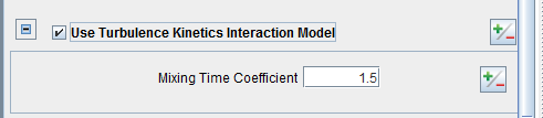
Turbulent Kinetics Interaction (TKI): Sub-cell scale turbulence chemistry interaction can be accounted for with the TKI model. This mixing time-scale model considers that the combustion chemistry should be partly controlled by the breakup of turbulent eddies due to the imperfect mixing of fuel and oxidizer in an actual engine process. The TKI model is recommended for use with high-load cases only, as for low-load cases the impact of the TKI model is expected to be much less. Also, the TKI model is recommended only for cases with in-cylinder fuel injection, for which the TKI model would consider the effects of imperfect mixing of fuel and oxidizer.
A value of 1.5 is recommended for the Mixing Time Coefficient setting under the TKI model. While a larger value of this input increases the turbulent mixing effect on reaction rates, a very high value would also suppress chemistry for post-injection expansion stroke conditions.
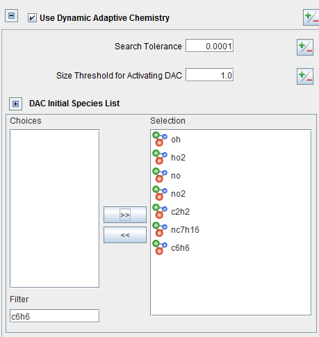
Dynamic Adaptive Chemistry (DAC): This option performs a mechanism reduction on the fly during the simulation. It should only be considered when there are 500+ species in the reaction mechanism. For the initial species, this includes all fuel species, important radicals (such as OH, HO2), NO, NO2, and soot precursor species (C2H2, soot). In Figure 4.16: Dynamic Adaptive Chemistry (DAC) panel, the fuel n-heptane (nc7h16), and the soot precursors acetylene (c2h2) and benzene (c6h6) are included.
For the Search Tolerance, the default value of 0.0001 is recommended. The Size Threshold for Activating DAC acts as a trigger for activating DAC. This value represents the ratio of species in the reduced mechanism to the number of species in the full mechanism. DAC will be enabled when this ratio is smaller than the threshold set here. A value of 1.0 will result in DAC being always enabled. Depending on the size of the full mechanism, this value can be set between 0 and 1.
Dynamic Cell Clustering (DCC): This option lumps together kinetically similar cells, therefore reducing the size of the chemistry problem to solve. This option should always be activated and the settings kept at the default.
Activate Chemistry: By default, chemistry is always solved, but this is not necessarily needed prior to injection or spark timing. Use the Conditionally option and activate the chemistry for the combustion event and afterwards only. You may activate chemistry after fuel injection or the first spark, use the Threshold Temperature option, and/or During Crank Angle Duration. These practices can help you save computational time.
Note: The chemistry activation controls using spark timing or injection timing will be ignored after the first engine cycle. Because of this, using controls based on crank-angle intervals for multicycle simulations is recommended. In a crank-angle-interval–based control, both the user-specified starting and ending crank angles will be converted to fit in the range of [0, 720) or [0, 360) CA degrees for four-stroke or two-stroke engines, respectively. The chemistry activation/deactivation events will consequently be examined in those engine cycle ranges.
Transport Terms
Typically, these never need to be adjusted. If you are having convergence issues, contact the Ansys support team at support@ansys.com.
Spatially Resolved Data
Spatially resolved data is written to every cell during the calculation. While the user specifies the frequency, it should be noted that the amount of disk space required will go up with a higher frequency. Typically, solutions are written every 10 CA degrees and the User Defined outputs option is used to write data out more frequently during important points in the cycle, such as injection, spark, combustion.
For File Size Control, there are three options:
One File: All the data is written to a single file. This is not the desired option since the file will become very large and this requires more time during file I/O and in rendering in the post-processor.
File Size: This option allows you to specify a file size in megabytes for the maximum file size before another file is written.
Solution Count: This is the best option since you can control how many solutions are written to a single file. A value of 1 means one solution per file. This is the preferred option.
Spatially Averaged Data
Spatially averaged data is data that is averaged over the domain. Since this is X-Y data, the data can be written more frequently, such as every 1 CA degree, or even more frequently.
Restart Data
Restart points can be written at certain frequencies in Forte. It is suggested a restart be written on the last simulation time-step, and also during the simulation prior to events occurring, such as Intake Valve Opening ("IVO"), start of injection, start of spark. You may specify the times to write out restart points.
Prior to submitting the simulation to the Forte solver, you should preview the motion of all the boundaries to be sure all the moving parts are moving correctly. In addition, it is suggested to preview the mesh before submitting the run. This will provide some information on the number of cells used and allow you to visualize the mesh to be sure it is not too coarse and not too fine. Some points of interest are: TDC, injection timing, spark timing, IVO, peak intake valve lift, Exhaust Valve Opening ("EVO").
During an IC engine simulation, there are certain points and items to check to ensure the best possible results are achieved. The following checklist can be used as a guideline:
Check CR compression ratio by running no-hydro case from -180 to 0 CA:
Three options are available to adjust compression ratio:
Clearance (squish) height.
Crevice width (for sector case, use between 1.0 and 1.5 mm, avoid a long skinny crevice).
Crevice height (can be adjusted for sector case).
Run simulation to Start-Of-Injection (SOI) or spark timing, check compression pressure:
Adjust intake pressure and temperature to match pressure at SOI or spark timing (scale both P and T by same %).
(If the compression pressure trace does not match the experimental data, refer to Mismatch of Compression Pressure.)
Check A/F ratio in the simulation vs. experimental:
Check IVC mass to be sure A/F ratio computed mass is consistent with P & T for the IVC condition for the sector case.
IVC total mass can be computed from the ideal gas equation.
If needed, adjust P or T up or down to match IVC mass.
Check ignition timing by looking at heat release rate (HRR):
Be sure you compare apparent HRR and NOT chemical HRR with engine data; apparent HRR takes heat losses (computed from P curve).
You can adjust SOI +/−1CA deg. (typical uncertainty) to match the ignition timing.
Check expansion pressure:
If expansion pressure is low, there could be several possible reasons:
Fuel amount is incorrect.
Too much heat transfer through the walls, typically the liner.
(If the expansion pressure trace does not match the experimental data, refer to Mismatch of Expansion Pressure.)
Check emissions:
NOx is very important; if NOx is not predicted accurately, there is little confidence in other emissions, such as soot.
NOx is highly dependent on temperature and can be dominated by local temperatures.