


The following sections of this chapter are:
This tutorial is divided into the following sections:
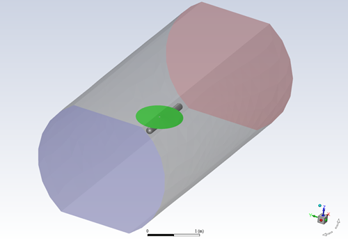
This tutorial provides guidelines for setting up and solving a simple helicopter simulation using Fluent’s Virtual Blade Model (VBM). The physical rotor is replaced with an actuator disk of finite thickness that provides the framework to simulate the thrust and torque of the actual rotor and to represent the rotor effects on the working fluid using the momentum source terms in Fluent’s governing equations. Local flow characteristics in the actuator disk are extracted from the 3D flow solution generated by Fluent and used by the VBM to compute the forces acting on each blade section from airfoil look-up tables, using Blade Element Theory (BET), then applied to the cells composing the actuator disk. Hence the unsteady rotor problem is replaced with a much simpler time-averaged procedure that can be used very effectively for the initial design of a real helicopter. The simplified helicopter geometry in this tutorial consists of a cylinder with a hemispherical nose and a flat disk to simulate the simple tethering rotor and rotor/fuselage flow interaction in the Georgia Institute of Technology (GIT) wind tunnel test chamber. The primary purpose of this tutorial is to illustrate the methodology for conducting this type of simulation, however, even though the mesh is very coarse, very reasonable agreement with the published experimental data can be obtained.
VBM meshing requirements.
Setting up and running in different scenarios.
Post-processing the different sets of results and interpreting the differences.
This tutorial will demonstrate the simulation of a simple helicopter in forward-flight in the Georgia Institute of Technology (GIT) wind tunnel [1-6] shown in Figure 34.1: Simple Helicopter in the GIT Wind Tunnel Test Section. The geometric and operating conditions are listed in Table 34.1: Geometric Data and Operating Conditions.
Table 34.1: Geometric Data and Operating Conditions
| Geometric Data | |
|---|---|
| Tunnel dimensions | 2.134 x 2.743 x 4.877 m |
| Body diameter | 0.134 m |
| Body length | 1.35 m |
| Body/rotor clearance | 0.135m |
| Rotor blades | 2 |
Rotor radius  | 0.4570 m |
| Cutout radius | 0.0125 m |
| Hinge offset | 0 m |
| Blade section | NACA 0015 |
| Blade chord | 0.086 m |
| Disk pitch angle | -6° |
| Disk bank angle | 0° |
| Collective pitch | 10° (fixed) |
| Coning angle | 0° |
| Longitudinal flapping angle | 1.94° |
| Lateral flapping angle | 2.03° |
| Blade twist | 0° |
| Operating Conditions | |
|---|---|
| Advance ratio (J) | 0.1 |
| Reference pressure | 101263.15 Pa |
| Reference temperature | 288.0997 K |
| Reference density | 1.22451 kg/m3 |
| Entrance velocity (Vx) | 10.04996 m/s |
| Rotational speed |
2,100 rpm (Ω = 219.9115 rad/s) |
| Tip speed | 100.49955 m/s |
For this simulation, the advance ratio is defined as:

For rotor simulations, operating cases will be considered using Embedded Disk Mode (EDM) at first:
No trimming
Collective trimming
Collective and cyclic trimming
Then, Floating Disk Mode (FDM) will be used to simulate a no-trimming option. Finally, the previous simulation will be performed restarting from a preset VBM case/data file.
The following sections describe the setup steps for this tutorial:
- 34.1.3.1. Preparation
- 34.1.3.2. Mesh
- 34.1.3.3. Enabling the Virtual Blade Model
- 34.1.3.4. Setup Units
- 34.1.3.5. Operating Conditions
- 34.1.3.6. Physical Modeling
- 34.1.3.7. Materials
- 34.1.3.8. Boundary Conditions
- 34.1.3.9. Reference Values
- 34.1.3.10. Discretization and Solution Controls
- 34.1.3.11. Solution Initialization
- 34.1.3.12. VBM Rotor Inputs
- 34.1.3.13. Convergence Monitoring
- 34.1.3.14. Post-processing Setup
- 34.1.3.15. Saving Settings and Re-Launching
To prepare for running this tutorial:
Download the
vbm_helicopter_tutorial.zipfile here .Unzip
vbm_helicopter_tutorial.zipto your working directory and ensure the following files are available:naca0015.dat
VBM_helicopter_tutorial.msh.gz
xnr_phi0.xy
xnr_phi090.xy
xnr_phi180.xy
xnr_phi270.xy
Use the Fluent Launcher to start Ansys Fluent.
Select Solution in the top-left selection list to start Fluent in solution mode.
Select 3D for , Double Precision for Solver Options and a suitable number of Processes.
Select the appropriate Working Directory in the General Options panel.
Click .
To read the mesh file, go to:
 → →
→ → Select the VBM_helicopter_tutorial.msh.gz file and click .
To display the mesh, click the following button in the ribbon.
Domain
→ Mesh → Deselect inlet, outlet and tunnel in the Surfaces list, select int_rotor and fuselage and click .
Since this case uses an embedded disk (EDM approach) in the first part of this tutorial, the computational domain must be divided into two separate but connected fluid domains (cell zones) (Physics → Zones → Cell Zones). The VBM only acts on the cells that form the live1 cell zone attached to one side of the actuator disk.
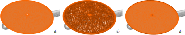
As shown in Figure 34.2: From Left to Right, the Three Components of the live1 Cell Zone: Int_Rotor, Int_live1 and Int_Live., Fluent automatically subdivides the live1 cells into three separate entities.
int_rotor contains the internal single-sided cell faces lying on the actuator disk surface,
int_live: contains the cell faces shared by the live and live1 domains, excluding the actuator disk,
int_live1 contains the internal cell faces perpendicular to the disk,
To display the first two surfaces, select each in the list of Surfaces, and click .
For the third surface, however, click Adjacency in the Mesh Display dialog box to open the Adjacency dialog box. Select live1 from the list of Cell Zone(s) and int_live1 from the list of the Adjacent Face Zones and then click on the Display Face Zones.
If this arrangement is not respected, the VBM will not work properly in Embedded Disk Mode.
Figure 34.2: From Left to Right, the Three Components of the live1 Cell Zone: Int_Rotor, Int_live1 and Int_Live.
Since this tutorial uses Embedded Disk Mode, the following mesh topology characteristics must be respected:
The entire 360˚ azimuth of the rotor must be modeled.
The actuator disk surface (int_rotor) must have the interior boundary condition.
The cells attached to one side of the disk must be marked as a separate domain (live1).
These cells must have one complete face attached to the disk. Only hexa and prisms are allowed.
A continuum fluid zone (live) must completely envelop the rotor zone (live1).
The fluid zone and rotor zone must have different BC index (id=13 for the fluid zone and 1 for the rotor zone).
Note: There is no need to create the disk and corresponding cell zone in the mesh when using Floating Disk Mode. Floating disks can be created during the VBM setup.
Fluent VBM can be enabled through the VBM Rotor Inputs dialog box or through the Text User Interface (TUI) by using the following text user interface command in the Fluent Console:
define/models/virtual-blade-model/enable?Answer yes when asked to enable the Virtual Blade Model.
Note: The VBM is only available with Dimension set to 3D.

The VBM can only be enabled when a valid Ansys Fluent case or mesh file has been set or read.
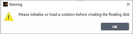
The current compatibility of the VBM is limited as it cannot operate with multiphase or inviscid flow. If any of these are active, Fluent will prevent the VBM from being enabled and display a warning message via either the Console or a pop-up message.
Since this tutorial is in the SI system of units and the rotor disk, blade pitch and blade flapping angles are provided in degree, go to:
![]() Domain
→ Mesh → Units...
Domain
→ Mesh → Units...
Click the si tab.
Click angle in the Quantities list and choose in the Units list.
Close the Set Units dialog box.
Set the operating conditions.
![]() Physics
→ Solver →
Physics
→ Solver →
Set a value of
101263.15Pa in the Operating Pressure box.Set the value of the X component of the Reference Pressure Location to -
1m.Click .
Configure the Fluent solver settings.
Physics
→ Solver → Select the following options in Task Page:
Type →
Velocity Formulation →
Time → Steady
Enable the energy equation.
Physics
→ Models → EnergyEnable the Energy box.
Select the turbulence model.
Physics
→ Models → Select the Spalart-Allmaras (1 eqn) turbulence model
Enable the Strain/Vorticity – Based production option.
Enable Viscous Heating and Curvature Correction in the Options section.
Click to accept all the other default settings and close the Viscous Model dialog box.
For vorticity-dominated flows, the default Vorticity-Based-production option overpredicts the production of eddy viscosity in the vortex cores. Adding the strain tensor to the vorticity reduces the production of turbulent viscosity in regions where the measure of vorticity exceeds that of strain rate.
This simulation features a high-speed flow regime, hence compressibility must be enabled.
![]() Physics
→ Materials →
Physics
→ Materials →
Select air as the working fluid in the pull-down menu
Select ideal-gas in the Density pull-down menu.
Click the Change/Create button.
Close the Create/Edit Materials dialog box.
Note: VBM also works with the constant density and incompressible-ideal-gas options. However since rotors usually operate in the compressible regime, the ideal-gas option is more appropriate.
Configure the boundary conditions.
![]() Physics
→ Zones →
Physics
→ Zones →
Set the boundary condition at the inlet.
Select the inlet boundary in the Task Page, ensure that its Type is velocity-inlet and click the button.
In the Momentum panel of the ribbon, select the Components option from the pull-down menu.
Select Absolute in the pull-down menu.
Input the values (
10.049955,0,0) m/s for the X-, Y- and Z-Velocity components, respectively.This velocity is calculated using the definition of the advance ratio J = 0.1.
In the Turbulence section, select the Intensity and Hydraulic Diameter option from the pull-down menu.
Set the Turbulence Intensity value to
1% (or Turbulence Intensity (fraction) value to0.01) and the Hydraulic Diameter value to0.134m. The diameter of the fuselage is assumed to represent the characteristic turbulent macroscopic length scale.In the Thermal panel of the ribbon, set a Temperature value of
288.0997K.Click and close the Velocity Inlet dialog box.
Set the boundary conditions at the outlet.
Select the exit boundary, ensure that the Type is , then click the button.
Select Absolute in the pull-down menu.
Set the Gauge Pressure value to
0PascalIn the Turbulence section, select the Modified Turbulent Viscosity option in the Specification Method pull-down menu.
Set a value of
0.0001(m2/s) in the Backflow Modified Turbulent Viscosity box. There is very little chance that backflow may occur, however it is good practice not to skip this operation.In the Thermal panel of the ribbon, set the Backflow Total Temperature to
288.15K.Click and close the Pressure Outlet dialog box.
Set wall boundary conditions.
Select the tunnel boundary and click the button.
In the Momentum panel of the ribbon, set the Shear Condition to Specified Shear with {
0.0.0} X-, Y- and Z-Components, respectively.In the Thermal panel of the ribbon, select Heat Flux in the Thermal Conditions and ensure that the Heat Flux value is
0W/m2.Click and close the Wall dialog box.
Retain the default setting for the fuselage boundary.
Set the reference values.
![]() Physics
→ Solver → Reference
Values…
Physics
→ Solver → Reference
Values…
Select inlet from the Compute from pull-down menu.
Set the Area value to
0.65612m2 (disk area).Set the Length Value to
0.086m (blade chord).Select live from the pull-down menu.
Set the discretization options.
![]() Solution
→ Solution →
Solution
→ Solution →
Use the pull-down menus to set the following options:
Scheme → SIMPLE
Gradient → Green-Gauss Node Based*
Pressure → PRESTO!**
Density → Second Order Upwind
Momentum → Second Order Upwind
Modified Turbulent Viscosity → First Order Upwind
Energy → Second Order Upwind
Pseudo Time Method →
Note: *The node-based averaging scheme is more accurate than the default cell-based scheme, especially on unstructured meshes, and most notably for triangular and tetrahedral meshes.
**The PRESTO! pressure discretization scheme is recommended for highly rotating flows.
Retain the default solver parameters:
Solution
→ Controls → Controls...
Initialize the solution from inlet boundary values.
![]() Solution
→ Initialization
Solution
→ Initialization
Select and click to open the Solution Initialization task page which provides access to further settings.
Select under the Compute from drop-down.
Set Reference Frame to .
Click the button.
Note: It is recommended to initialize the solution before configuring the VBM rotor. Although a mandatory step for Floating Disk Mode due to use of Fluent post-processing tools for creating a floating disk, it can be delayed for Embedded Disk Mode.
Set up the VBM rotor.
![]() Physics
→ Models → More
Physics
→ Models → More
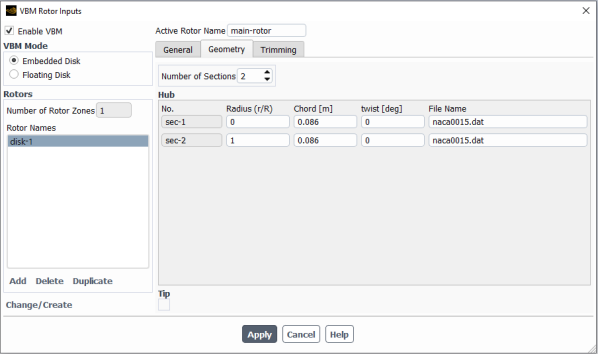
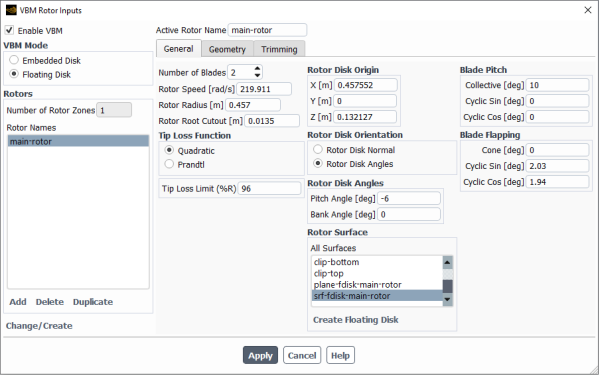
Select to open the VBM Rotor Inputs dialog box.
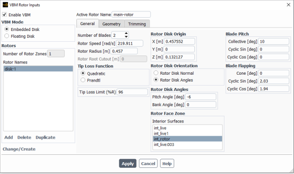
Toggle .
Select under VBM Mode.
Press . A new rotor with a default name disk-1 with default properties will be created. The settings appearing to the right will be updated in the next steps.
Enter
main-rotorin the Active Rotor Name box.Enter the parameters shown in Figure 34.3: General Disk Data Configuration Window.
Select int_rotor from the Interior Surfaces list to select the actuator disk surface.
Click the tab and enter the parameters shown in Figure 34.3: General Disk Data Configuration Window.
Click to save the settings. Click if the following warning message appears:
Click to close the VBM Rotor Inputs dialog box.
Note: The button must be clicked to save the updated entries of the current rotor before moving on to the next rotor or before pressing the button. This sequence must always be respected, even if the VBM Rotor Inputs dialog box (VBM graphical user interface) is re-opened to simply edit a parameter.
When pressing , Fluent VBM reads and pre-processes data entered in the VBM Rotor Inputs dialog box and reports information regarding each rotor zone.
VBM will append the .dat suffix to the airfoil file names if it is omitted in the VBM graphical user interface.
Consult Airfoil File Format within the Fluent User's Guide for more information on the geometry of the rotor blades and the effect of the parameters.
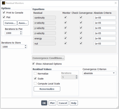
Configure the residuals monitors that will appear in the Fluent graphics window and console.
![]() Solution
→ Reports →
Solution
→ Reports →
Ensure that and options are enabled in the Options group box.
Enable and select from the Convergence Criterion drop-down list.
Set the Absolute Criteria values to
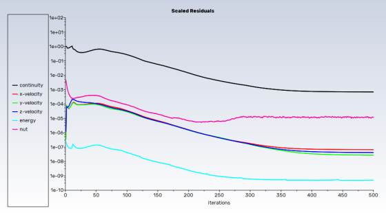
1e-6for Energy equation and to1e-5for other equations as shown in Figure 34.5: Solution Residuals Configuration.Click to close the Residual Monitors dialog box.
Additionally, you may also want to monitor pressure convergence on the actuator disk int_rotor. Go to:
![]() Solution → Reports
→ Definitions →
→ →
Solution → Reports
→ Definitions →
→ →
Enter
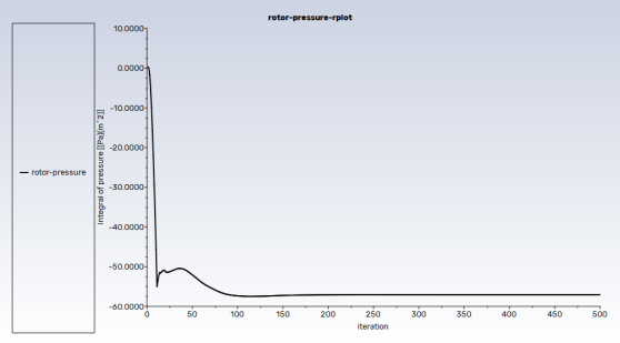
rotor-pressurein the Name box.Enable Report File, Report Plot and Print to Console in the Create section.
Select Pressure… and Static Pressure with the pull-down menus in the section.
Select in the Surfaces section.
Click to close the Surface Report Definition dialog box.
When the calculation begins, the pressure convergence history will be displayed in the Graphics window, printed in the Console and written in rotor-pressure-rfile.
Additionally, the convergence histories of the thrust, torque, power, moments and forces are written to the Rotor_1_Loads.dat file. If you want to see the convergence histories of any output quantity (for example, VBM Thrust) for the rotor, go to:
![]() Solution → Reports
→ Definitions →
→ →
Solution → Reports
→ Definitions →
→ →
Enter
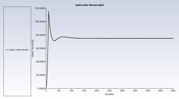
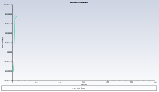
main-rotor-thrustin the Name box.Enable , and under .
Select under Report Type.
Select under Output Type.
Select main-rotor under Rotor Names.
Click to close the VBM Report Definition dialog box.
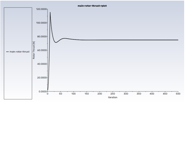
When the calculation begins, the rotor thrust convergence history will be displayed in the Graphics window, printed in the Console and written in main-rotor-pressure-rfile.out.
Example 34.1: The ribbon at the top of the Graphics window can be used to change the view options defined above.
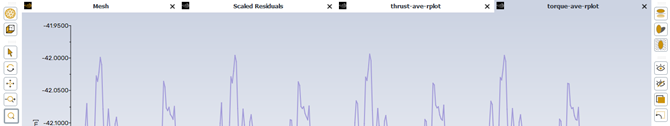
(residual/pressure-integral/rotor-thrust convergence history)
It's recommended to set up and save the post-processing configuration before proceeding with the actual solution process. Nevertheless, if you prefer, you may skip this section and configure the post-processing setup later after obtaining the solution. In the upcoming sections, you'll learn how to establish a framework for post-processing and extracting data from the solution. This framework will enable you to compare the solution data with experimental data.
Create two cutting planes to visualize the rotor-fuselage interaction. One cutting plane will be oriented perpendicular to the centerline of the fuselage, and the other one will be parallel to the centerline of the fuselage. These cutting planes will enable a comparison of the effect of trimming on the solution with and without trimming. Go to:
![]() Results → Surface
→ Create →
Results → Surface
→ Create →
The Plane Surface panel is shown in Figure 34.6: Create Plane Surface Plane-y=0.
Create plane-y=0
Enter
plane-y=0in the New Surface Name box.Select from the Method drop-down list and enable the box in the Options list. This will allow the creation of a bounded cutting plane using three corner points.
Enter the coordinates of the corner points in the Points section: P(1) = {
-0.25,0,-0.40}, P(2) = {1.5,0,-0.40} and P(3) = {1.5,0,0.70}.Click the button.
To define the next plane, do not close the Plane Surface dialog box.
Create plane-x=0.3

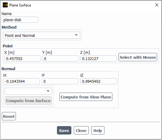
To properly visualize the VBM results, it's necessary to have a plane surface that intersects the entire rotor cell zone as VBM variables are cell-based. You will need to determine the surface normal vector and a point on the plane to create it. For this purpose, you may utilize the Rotor Disk Normal and Rotor Disk Origin.
![]() Results → Surface
→ Create →
Results → Surface
→ Create →
The Plane Surface panel is shown in Figure 34.7: Create Plane Surface Plane-Disk.
Enter
plane-diskin the New Surface Name box.Select under the Method drop-down list.
Enter the coordinates of the point in the Point section: {
0.457552,0,0.132127}Enter the normal vector components in the Normal section: {
-0.104528,0,0.996195}Click the button.
Close the Plane Surface dialog box.
Four curves will be created along the port and starboard sides and at the top and bottom of the cylindrical fuselage to enable the extraction of the pressure coefficient. The curves are saved so that they can be reused for the subsequent cases. Go to:
![]() Results → Surface
→ →
Results → Surface
→ →
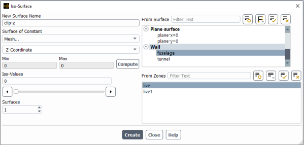
The Iso-Surface panel is shown in Figure 34.8: Iso-Surface Creation Panel.
Create clip-z.
Enter the name
clip-zin the New Surface Name box.Select Mesh… and then Z-Coordinate from the Surface of Constant drop-down list.
Select fuselage in the From Surface list and live in the From Zones list.
Set the Iso-Values to
0m.Click the button.
This operation creates a curve at the intersection of the cylindrical fuselage and an X-Y cutting plane at position Z = 0 m.
To define the next curve, do not close Iso-Surface dialog box.
Create clip-y.
Name the curve around the fuselage
clip-yin the New Surface Name box.Select Mesh… and then Y-Coordinate in the drop-down list.
Select fuselage in the From Surface list and live in the From Zones list
Set the Iso-Values to
0m.Click the button.
Close the Iso-Surface dialog box.
This operation creates a curve at the intersection of the cylindrical fuselage and an X–Z cutting plane at position Y = 0 m.
Create clip-port.
The curves created in the previous steps are irrelevant in their current state; they must be divided into port and starboard, top and bottom sides. Go to:
Results →
Surface →
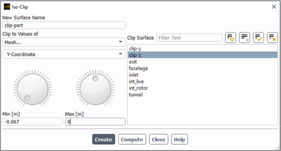
→ .The panel is shown in Figure 34.9: Iso-Clip Panel for the Creation of the Clip-Port Curve.
Enter the name
clip-portin the New Surface Name box.Select clip-z in the Clip Surface list.
Select Mesh… and then Y-Coordinate in the pull-down menus.
Click the button. The maximum and minimum Y limits of the curve clip-z are displayed under the two circular dials.
Change the Max [m] limit to
0and press the Enter key.Leave the Min [m] value at
-0.067.Click the button.
To define the next curve, do not close the Iso-Clip dialog box.
Create clip-starboard.
Enter the name
clip-starboardin the New Surface Name box.Retain clip-z in the Clip Surface list.
Click the button again.
Change the Min [m] to
0and press the Enter key.Leave the Max [m] value at
0.06699026.Click the button.
To define the next curve, do not close the Iso-Clip dialog box.
Create clip-bottom.
Enter the name
clip-bottomin the New Surface Name box.Select clip-y in the Clip Surface list.
Select Mesh… and then Z-Coordinate in the pull-down menus.
Click the button. The maximum and minimum Z limits of the curve clip-y are displayed under the two circular dials.
Change the Max [m] limit to
0and press the Enter key.Leave the Min [m] value at
-0.06693347.Click the button.
To define the next curve, do not close the Iso-Clip dialog box.
Create clip-top.
Enter the name
clip-topin the New Surface Name box.Retain clip-y in the Clip Surface list.
Click the button again.
Change the Min [m] to
0and press the Enter key.Leave the Max [m] value at
0.06698362.Click the button.
Close the Iso-Clip dialog box.
Delete clip-y and clip-z.
The clip-y and clip-z curves are no longer needed and therefore can be deleted. Go to:
Results → Surface → Manage…
Select clip-y and clip-z in the Surfaces list and click the button.
the Surfaces dialog box.
The experimental pressure coefficient data is provided with respect to the normalized x-coordinate x/r, where r is the radius of the rotor. Therefore it is necessary to define a Custom Field Function to facilitate direct comparison.
![]() User-Defined → → Custom…
User-Defined → → Custom…
Select Mesh… and then X-Coordinate in the pull-down menus. Click the button. An x will appear in the Definition box.
Click the button.
Enter the value
0.457with the keys of the numeric keypad, as shown in Figure 34.10: Custom Field Function Configuration Panel.Enter the name
x-normin the New Function Name box.Click the Define and buttons.
Note: To change/modify an already defined custom field function, click the button.

Before launching the simulation, it is recommended to save your work. Go to:
![]() →
→
→
→
and save the settings to the VBM_helicopter_tutorial.cas
file. Alternately, ![]() →
→ can be used if you want to save both case and data
file.
→
→ can be used if you want to save both case and data
file.
You can exit Fluent by selecting ![]() →
or by clicking the X icon in
the top right corner of the application. Otherwise, go to Solution to run calculation.
→
or by clicking the X icon in
the top right corner of the application. Otherwise, go to Solution to run calculation.
If you exit Fluent, the steps below should be followed to re-launch and apply VBM before running calculations.
Launch the Fluent executable in the working directory using the same launching setup shown in Preparation.
Read the case file,
File →
Read → Case... and
select VBM_helicopter_tutorial.cas. Alternatively,
you can read both case & data file when restarting from a previous
solution.Initialize the solution from inlet boundary values, select
Solution →
Initialization →
Initialize. If you restarted from a previous
solution, you can skip this step.Apply the VBM, select
Physics →
Models → More →
to open the VBM
Rotor Inputs dialog box and click
. This action will prompt the Fluent VBM
to read and pre-process rotor setup in the VBM Rotor
Inputs dialog box and report details on each rotor
zone.
Five simulations will be executed to demonstrate the capabilities of the VBM:
- 34.1.4.1. Rotor Simulation with Fixed-Pitch Using EDM
- 34.1.4.2. Rotor Simulation with Collective Trimming
- 34.1.4.3. Rotor Simulation with Collective and Cyclic Trimming
- 34.1.4.4. Rotor Simulation With Fixed Pitch Using FDM
- 34.1.4.5. Rotor Simulation Restarting From a VBM Case/Data File
- 34.1.4.6. Comparison with Experimental Results
For the first simulation, the helicopter rotor is operating in fixed-pitch mode without trimming using the EDM approach. Go to:
Solution → Run
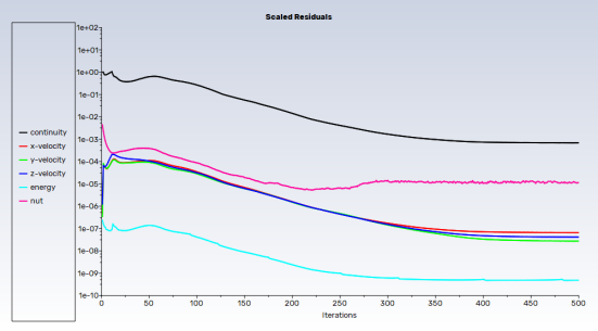
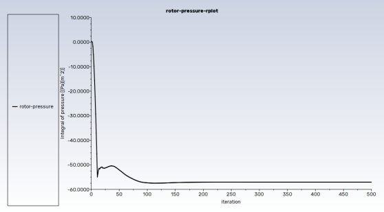
Calculation → Run Calculation... Set the No. of Iterations value to
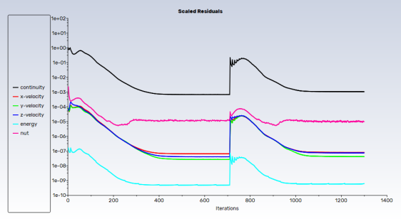
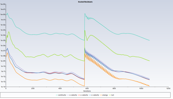
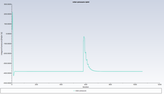
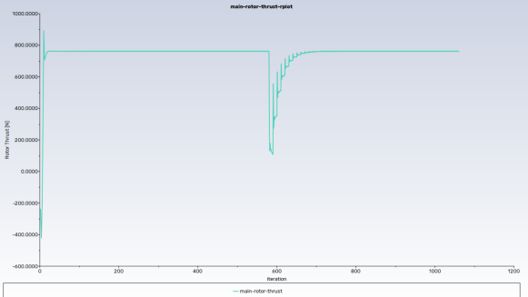
500and click the button.The convergence history of the residuals is shown in Figure 34.11: Convergence History. Figure 34.12: Pressure Monitor Convergence History shows the convergence history of the integral of the static pressure on the int_rotor surface. The convergence history of the main-rotor thrust, which is a VBM output quantity, is demonstrated in Figure 34.13: Rotor Thrust Monitor Convergence History. It can be observed that the main-rotor thrust converged more quickly than the residuals, although this is not always the case.
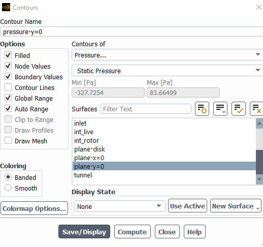
To display contours of pressure on the cutting planes that have been created in Cutting Planes for the Pressure Distributions, go to:
Results →
Graphics →
→ Configure the window as shown in Figure 34.14: Pressure Distribution Contours on the Y=0 Plane.
Click the button to display the image in the graphics window.
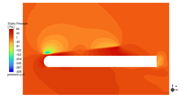
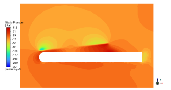
To see the contours on plane-y=0, as shown in Figure 34.15: Pressure Distribution with Fixed Blade Pitch, Y=0 Cutting Plane, click the green y-axis arrow in the axis triad twice and click the button in the graphics toolbar.
To change the colormap, click to open the Colormap dialog and set the parameters (Number Format, Font Size, Colormap Size, etc) based on your preference.
To disable the light on the contour, go to the Lights dialog box, and de-select :
View →
Graphics →
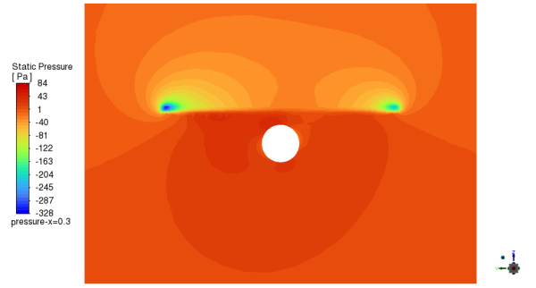
Create a similar contour for the plane-x=0.3 to see the image of Figure 34.16: Pressure Distribution with Fixed Blade Pitch, X=0.3 Cutting Plane. Use the axis triad, rotation controls, and Lights dialog box as needed.
Figure 34.15: Pressure Distribution with Fixed Blade Pitch, Y=0 Cutting Plane and Figure 34.16: Pressure Distribution with Fixed Blade Pitch, X=0.3 Cutting Plane show that there is a clear pressure load imbalance on the disk, therefore if the helicopter were free to fly, it would not be able to maintain a straight-and-level course, rather it would tilt up and roll to the left. To achieve stability, the rotor must be trimmed so that the pressure integrated over the rotor produces no net moments, only lift and thrust in the forward direction. This can only be achieved by fine-tuning the rotor collective and cyclic pitch (thrust and moment trimming).
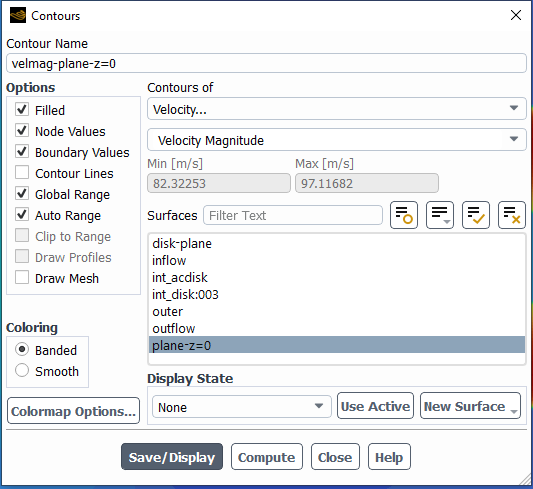
To display contours of your results on the disk planes that have been created in Cutting Planes for the VBM Results, go to:
Results →
Graphics →
→
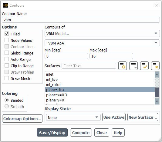
New...Configure the window as shown in Figure 34.17: Setup Contours to Display the Vbm AoA Distribution for Main-Rotor.
Ensure and all other options are deselected in the Options group box, with the exception of .
Note: The VBM variables are cell-based. Therefore must be de-selected for the values to display correctly.
Click the button to display the image in the Graphics window.
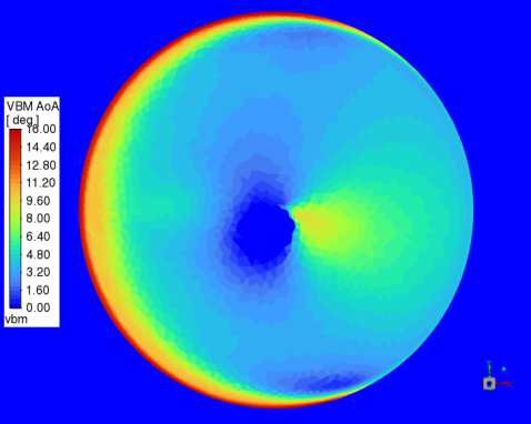
Modify , rotate the view and zoom in to get the display shown in Figure 34.18: VBM AoA Distribution for Main-Rotor
Press Compute. The AoA distribution is in the range of -79.97 to 16.77 degrees. During forward flight, the retreating blade experiences a reduction in the relative airflow velocity and can enter a stall condition (positive or negative AoA with an absolute magnitude larger than stall angle), where the airflow separates from the blade surface and creates a region of reverse flow.
Try different VBM variables and visualize their contours by displaying them.
Save the Fluent case and data files (VBM_helicopter_tutorial.cas and VBM_helicopter_tutorial.dat):
File → Write
→
The next simulation should be identical to the previous one, with the exception that, now, the VBM model will trim the collective angle of the rotor. It is expected that the trimming will recover the exact blade pitch angle of the fixed-pitch rotor and produce the same thrust. Before enabling the collective trimming, the thrust coefficient of the fixed-pitch rotor must be computed from the fixed-pitch solution with the following equation:

Table 34.2: Values from the Fixed-Pitch Solution lists the values of the
variables appearing in the formula. The rotor thrust  can be recovered from column 3 of the last line of the VBM log
file Rotor_1_Loads.csv.
can be recovered from column 3 of the last line of the VBM log
file Rotor_1_Loads.csv.  is the coefficient of the dynamic pressure set to 1 in the
code. The blade tip velocity and the reference density are listed in Table 34.1: Geometric Data and Operating Conditions.
is the coefficient of the dynamic pressure set to 1 in the
code. The blade tip velocity and the reference density are listed in Table 34.1: Geometric Data and Operating Conditions.
Table 34.2: Values from the Fixed-Pitch Solution
| Variable | Value | |
|---|---|---|
 | rotor thrust | 74.94955 N |
 | dynamic pressure coefficient | 1 |
 | blade tip velocity | 100.499327 m/s |
 | reference density | 1.22451 kg/m3 |
 | rotor diameter | 0.914 m |
The computed thrust coefficient value CT is 0.0092363.
To enable collective trimming, go to:
Physics →
Models → Select to open the VBM Rotor Inputs dialog box.
Select the Trimming panel in the ribbon and enable Collective pitch.
Set the Update Frequency value to
10, the Damping Factor to0.7and enter the value0.0092363in the Desired thrust coefficient box.Click the button to save the new entries.
Press the button to pre-process the VBM inputs.
To run the calculation, go to:
Solution →
Set a value of
200in the No. of Iterations box and press the button.The residuals, pressure and thrust monitor values should not change for the next 200 iterations. This short run is required only to verify that the thrust coefficient value is precise and the collective angle printed to the Console after 200 iterations converges to the original 10° fixed-pitch blade angle.
When the execution terminates, save the case and data files (VBM_helicopter_tutorial_VP.cas and VBM_helicopter_tutorial_VP.dat).
→
→
To enable cycling trimming, go to:
Physics→
Models → Select to open the VBM Rotor Inputs dialog box.
Select the Trimming option in the ribbon and enable the Cyclic pitch option.
Enter the value
0in the Desired pitch-moment coefficient and Desired roll-moment coefficient boxes.Click the button, then press the button.
To run the calculation, go to:
Solution→
Set a value of
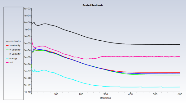
600in the No. of Iterations box and press the button.At convergence the residual history will look like Figure 34.19: Convergence History with Collective and Cyclic Angles Trimming.
When the execution terminates, save the case and data files (VBM_helicopter_tutorial_Co_Cy.cas and VBM_helicopter_tutorial_Co_Cy.dat):
→
→ During the saving process, trimming results will also be saved in a Fluent .dat file and printed in the Console. Due to cyclic pitch trimming, the collective pitch angle changes to 10.14838˚ and the coefficient of cyclic cosine and sine components of the blade pitch angle change to -1.91224˚ and 2.83469˚, respectively. The resulting converged rotor thrust with both collective and cyclic trimming is still 74. 94954 N, as it was prior to trimming. These values can be found in the third column of the Rotor_1_Loads.csv output file.
Figure 34.20: Pressure Distribution with Collective and Cyclic Trimming, Y=0 Cutting Plane and Figure 34.21: Pressure Distribution with Collective and Cyclic Trimming, X=0.3 Cutting Plane show that the cyclic trimming has balanced the pressure distribution almost equally along, and especially across, the rotor.
Exit Fluent by selecting in the ribbon tab or by clicking the X icon in the top right corner of the application. For the latter, a Warning dialog box will open. Press to exit Fluent.

Previous simulations were performed using Embedded Disk Mode. In this section, Rotor Simulation with Fixed-Pitch Using EDM is repeated using Floating Disk Mode. The difference is related to the rotor input setup, such that a floating disk is used instead of an embedded disk. This tutorial begins by reading the case file saved in the first simulation and then changing some settings. Generally, the mesh has less prerequisites for the VBM with a floating disk. In this case, the same grid is used for consistency.
If not already done, exit Fluent. Create a new working directory and copy VBM_helicopter_tutorial.cas and naca0015.dat to this new directory.
Launch the Fluent executable in the new working directory using the same launching setup as Preparation.
To re-read the case file, go to:
→
→ and select VBM_helicopter_tutorial.cas.
Initialize the solution from inlet boundary values. Go to:
Solution →
Initializationand click the button.
Note: Before creating the floating disk, an initial solution should be loaded or initialized. Otherwise, Fluent will give a warning message to do so.
To set up the rotor parameter, go to:
Physics →
Models → MoreSelect to open the VBM Rotor Inputs dialog box.
Select Floating Disk as the VBM Mode.
Set Rotor Root Cutout [m] to
0.0135.Retain all other settings as shown in Figure 34.22: General Disk Data Configuration Window, FDM, Fixed Pitch.
Press . Fluent will create and select the Rotor Surface named srf-fdisk-main-rotor.
Click to save the settings.
Click in the Warning dialog box that appears stating that trimming is off.
Click to close the VBM Rotor Inputs dialog.
To run calculation, go to:
Solution → Run
Calculation → Run
Calculation...Set the No. of Iterations to
500and click .The convergence history of the residuals is shown in Figure 34.23: Convergence History, FDM, Fixed Pitch. Figure 34.24: Pressure Monitor Convergence History, FDM, Fixed Pitch also shows the convergence history of the integral of the static pressure on the int_rotor surface. In addition, the convergence history of the main-rotor thrust is demonstrated in Figure 34.25: Rotor Thrust Monitor Convergence History. As shown in the pictures, the converging history of the current simulation using FDM is similar to that of using EDM (see Rotor Simulation with Fixed-Pitch Using EDM).
In general, VBM simulations using FDM and EDM should yields the same results as long as the meshes and facets on the disks are the same. In the current simulation, the converged global rotor results are almost the same as those of EDM approach, as shown in Table 34.3: Comparison Between Global Rotor Results Obtained Using EDM and FDM. The negligible discrepancies in the results are due to the difference between the embedded and floating disk’s facets.
Table 34.3: Comparison Between Global Rotor Results Obtained Using EDM and FDM
Thrust [N] Torque [Nm] Power [W] Roll Moment
[Nm]
Pitch Moment [Nm] Xp Force
[N]
Yp Force
[N]
EDM 74.94955 -2.512792 552.5905 3.40641 -3.234057 2.75369 0.8662077 FDM 74.97936 -2.513915 552.8376 3.423004 -3.218962 2.760432 0.8625094 When the execution terminates, save the case and data files (VBM_helicopter_tutorial_FDM.cas and VBM_helicopter_tutorial_FDM.dat):
File → Write
→ Case & DataExit Fluent by selecting in the ribbon tab or by clicking the button in the top right corner of the application. For the latter, a Warning dialog box will open to confirm, press to exit Fluent.
The VBM case and data file includes VBM set-up and solutions. To re-launch a VBM case and restart from a previous saved data file, some steps are required. In this section, case/data files of previous simulation will be read to continue the simulation.
Read the case data files.
→
→ and read the VBM_helicopter_tutorial_FDM.cas and .dat files.
Display floating disk surface and srf-fdisk-main-rotor. Go to:
Domain → Mesh
→ and select srf-fdisk-main-rotor in the list of Surfaces and click . If this step is neglected, the VBM will not recognize the floating disk, potentially leading to it crashing.
To read and pre-process VBM data.
Physics →
Models → Select to open the VBM Rotor Inputs dialog box. Ensure srf-fdisk-main-rotor is selected from the list of Rotor Surface and press to perform the VBM pre-processing.
Run the calculation.
Solution → → Set the No. of Iterations to
100and click .Based on your preference, answer
yesornowhen asked to create the rotor-pressure-rfile.out and main-rotor-thrust-rfile.out report file. These report files were defined to monitor convergence history of surface pressure integral on the int_rotor surface and the thrust force on main-rotor. Answeryesif asked to overwrite these files in case you do not want to create new files.The convergence history of the residuals is shown in Figure 34.23: Convergence History, FDM, Fixed Pitch. As shown in the pictures, residuals continue with the same trends as re- siduals of the previous simulation (Rotor Simulation With Fixed Pitch Using FDM. The converged rotor thrust, 74.97935 N, listed in column 3 of the Rotor_1_Loads.csv log file, is also the same as that of in the previous simulation. Therefore, there is no need to save the case data files since the results obtained with 500 iterations in the previous simulation was sufficient.
Note: In the current release, post-processing tools in Fluent are used to create floating disk and the list of corresponding cells. Therefore, step-2 is required to create the list of VBM cells cut by the floating disk when reading a new data file or initializing the solution. Alternatively, you can create a new floating disk through the VBM Rotor Inputs dialog box. If this step is neglected, the VBM will not recognize the floating disk, potentially leading to it crashing.
For mode, there is no need to perform step 2 since all cells corresponding to embedded disk are marked in the mesh as a separate cell zone.
Even though the purpose of this tutorial is to illustrate the usage of Fluent VBM and the computational grid is rather coarse to keep the execution times as low as possible, the computational results can be compared to the experimental data for validation.
To re-read the case and solution files, go to:
→
→ and read the VBM_helicopter_tutorial.cas and VBM_helicopter_tutorial.dat files.
To compare the results along the top and bottom sides of the fuselage, using the XY plot panel, go to:
Results→
Plots→ → Deselect the Position on X Axis in the Options section.
Select Pressure and then Pressure Coefficient from the Y Axis Function pull-down menu.
Select Custom Field Functions… and then x-norm from the X Axis Function pull-down menu.
Select clip-bottom and clip-top in the Surfaces list.
Click the button and select the files: xnr_phi0.xy and xnr_phi180.xy containing the experimental data, then click .
Click the button.
It is possible to change curve style. Click Curves in the Solution XY Plot dialog box, then select the curve # and define the Line Style and Marker Style from the options in the Curve – Solution XY Plot dialog box.
To compare the results along the port and starboard sides of the fuselage:
Select the two files in the File Data list and click the button.
Deselect the clip-top and clip-bottom entities in the Surfaces list. Select clip-port and clip-starboard in the Surfaces list.
Click the button and select the xnr_phi090.xy and xnr_phi270.xy files containing the experimental data, the click .
Click the button.
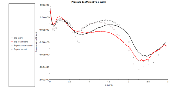
Figure 34.27: Pressure Coefficient Distribution Along the Top and Bottom of the Fuselage shows the comparison of the numerical and experimental pressure coefficient along the top and bottom of the fuselage. Figure 34.27: Pressure Coefficient Distribution Along the Top and Bottom of the Fuselage shows the comparison of the numerical and experimental pressure coefficient distribution along the port and starboard sides of the fuselage.

The same procedures can be used to compare the numerical results with collective and cyclic trimming to the experimental pressure coefficient along the fuselage. Go to:
![]() → →
→ →
and re-read the VBM_helicopter_tutorial_Co_Cy.cas and VBM_helicopter_tutorial_Co_Cy.dat files, then follow the same procedure outlined above.
Figure 34.29: Pressure Coefficient Distribution Along the Top and Bottom of the Fuselage Obtained with Collective and Cyclic Trimming shows the comparison of the numerical and experimental pressure coefficient along the top and bottom of the fuselage. Figure 34.30: Pressure Coefficient Distribution Along the Port and Starboard Sides of the Fuselage Obtained with Collective and Cyclic Trimming shows the comparison of the numerical and experimental pressure coefficient along the port and starboard sides of the fuselage.
Figure 34.29: Pressure Coefficient Distribution Along the Top and Bottom of the Fuselage Obtained with Collective and Cyclic Trimming
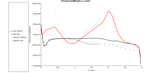
Figure 34.30: Pressure Coefficient Distribution Along the Port and Starboard Sides of the Fuselage Obtained with Collective and Cyclic Trimming
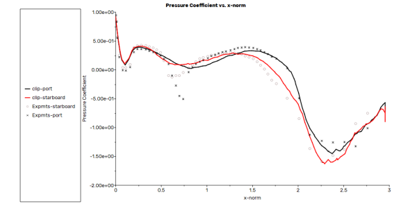
Some improvements in the agreement between the experimental and numerical results with collective and cyclic trimming are seen at the top of the fuselage. The numerical results on the port and starboard side have also improved considerably.
This tutorial explains the usage of Fluent’s VBM for a generic helicopter case and compares the numerical results with fixed blade pitch and with collective and cyclic trimming to the published experimental data.
Step-by-step instructions for the Fluent and VBM set up are provided to enable you to conduct realistic rotorcraft simulations.
The comparison of the fixed-pitch results with the collective trimming case implicitly demonstrates that the VBM trimming routine is stable and accurate.
Considering the coarseness of the grid, which has been tailored towards portability, simplicity and fast turnaround of the tutorial runs, rather than accuracy, a very reasonable agreement between the results of the simulation obtained with collective and cyclic trimming and the experimental data has been demonstrated.
VBM simulations using FDM and EDM for the same mesh and same conditions yield the same results.
Liou, S.G., Komerath, N.M. and McMahon, H.M. “Velocity Measurements of Airframe Effects on a Rotor in Low-Speed Forward Flight”, AIAA Journal of Aircraft, vol. 26, no. 4, 1989.
Glauert, H. “The Elements of Aerofoil and Airscrew Theory,” Second Edition, Cambridge University Press, New York, USA, 1947.
Stepniewski, W.Z. and Keys, C.N., “Rotary-Wing Aerodynamics,” Dover Publications Inc., New York, USA, 1984.
Leishman, J.G., “Principles of Helicopter Aerodynamics,” Cambridge University Press, New York, USA, 2000.
Zori, L.A.J., Rajagopalan, R.G., “Navier-Stokes Calculation of Rotor-Airframe Interaction in Forward Flight”, Journal of the American Helicopter Society, Vol.40, April 1995.
Brand, A.G., Komerath, N. and McMahon, H., “Results from Laser Sheet Visualization of a Periodic Rotor Wake”, AIAA Journal of Aircraft, vol. 26, no. 5, 1989.
Liou, S.G., Komerath, N.M. and McMahon, H.M. “Velocity Field of a Cylinder in the Wake of a Rotor in Forward Flight”, AIAA Journal of Aircraft, vol. 27, no. 9, 1990.
Liou, S.G., Komerath, N.M. and McMahon, H.M. “Measurements of the Interaction Between a Rotor Tip Vortex and a Cylinder,” AIAA Journal, vol. 28, no. 6, 1990.
D.N. Mavris, Komerath, N.M. and McMahon, H.M. “Prediction of Aerodynamic Rotor-Airframe Interactions in Forward Flight”, Journal of the American Helicopter Society, October 1989.
Brand, A.G., Komerath, N.M. and McMahon, H.M., “Windtunnel Data From a Rotor Wake/Airframe Interaction Study”, Georgia Institute of Technology, US Army Research Contract No. DAAG 29-82-K-0094, 1986.
This tutorial is divided to the following sections:
This tutorial provides guidelines for setting up and solving flow on a 6-bladed aircraft propeller using Fluent’s Virtual Blade Model (VBM). The physical propeller is replaced with an actuator disk of finite thickness that provides the framework to simulate the thrust and torque of the actual propeller using the momentum source terms in Fluent’s governing equations. Local flow characteristics in the actuator disk are extracted from the 3D flow solution generated by Fluent and used by the VBM to compute the forces acting on each blade section from airfoil look-up tables, then applied to the cells composing the actuator disk. The unsteady propeller problem is replaced with a much simpler time-averaged procedure that can be used very effectively for the initial design of a real propeller-driven aircraft. Although the mesh is very coarse, the purpose of this tutorial is to illustrate the methodology for conducting this type of simulation, rather than as a validation of the Virtual Blade Model that should be conducted with much finer grids.
Although the VBM has been specifically developed for rotorcraft simulations, it is also applicable to general rotating machinery (propellers, wind power, HVAC, automotive, marine, etc.), for flows typically characterized by:
Low-to-moderate blade loading
Predominantly axial flow
Negligible geometrical blockage
This tutorial will cover the following topics:
VBM meshing requirements.
Setting up and running a test case using the VBM.
Running a fixed-pitch and thrust-trimmed simulation.
Post-processing the two sets of results and interpreting the differences.
This tutorial will demonstrate the simulation of a simple propeller modeled by an actuator disk, as shown in Figure 34.31: Simple Propeller, Modeled by an Actuator Disk (Green), Inside a Cylindrical Domain. The geometric and operating conditions are listed in Table 34.4: Propeller Geometric Data and Operating Conditions.
Table 34.4: Propeller Geometric Data and Operating Conditions
| Geometric Data | |
|---|---|
| Tunnel dimensions | 50 x 30 m |
| Tunnel turbulence intensity | 1% |
| Rotor blades | 6 |
| Rotor radius | 0.5 m |
| Cutout radius | 0.15 m |
| Hinge offset | 0 m |
| Blade section | NACA 16016 (6% camber) |
| Blade root chord | 0.1 m |
| Blade tip chord | 0.05 m |
| Disk pitch angle | -90° |
| Disk bank angle | 0° |
| Collective pitch angle | 61.85345° (fixed) |
| Coning angle | 0° |
| Longitudinal flapping angle | 0° |
| Lateral flapping angle | 0° |
| Blade twist | -35.12931° |
| Operating Conditions | |
|---|---|
| Design advance ratio (Jd) | 1.4208 |
| Reference pressure | 97013.91 Pa |
| Reference temperature | 284.5926 K |
| Reference density | 1.187584 kg/m3 |
| Inflow velocity (Vx) | 84.54519 m/s |
| Rotational speed |
3570.321 rpm (373.8831 rad/s or 59.50536 rev/s) |
| Tip velocity | 186.94155 m/s |
The conditions in Table 34.4: Propeller Geometric Data and Operating Conditions were computed using the following definition of the advance ratio.

where
 – propeller diameter (m)
 – rotational speed (rev/s)
 – rotational speed (rad/s)
 – propeller axial flow velocity (m/s)
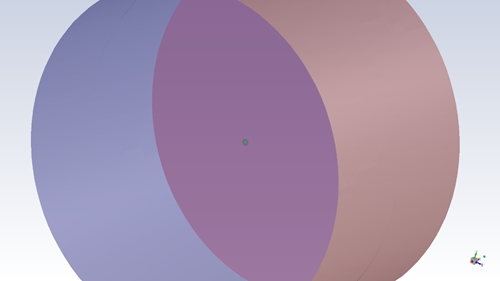
Table 34.5: Geometric Characteristics of the Propeller Blade
| Section | r/R | Chord [m] | Twist [deg] | Airfoil |
|---|---|---|---|---|
| 0 | 0.30 | 0.100000 | 0.00000 | naca16016 |
| 1 | 0.40 | 0.098922 | -6.55173 | naca16016 |
| 2 | 0.50 | 0.095905 | -12.11207 | naca16016 |
| 3 | 0.60 | 0.090733 | -17.06897 | naca16016 |
| 4 | 0.70 | 0.083621 | -21.16379 | naca16016 |
| 5 | 0.80 | 0.074353 | -24.91379 | naca16016 |
| 6 | 0.90 | 0.063308 | -28.53448 | naca16016 |
| 7 | 0.95 | 0.056519 | -30.99138 | naca16016 |
| 8 | 1.00 | 0.050000 | -35.12931 | naca16016 |
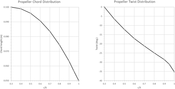
The geometric characteristics of the propeller blade are listed in Table 34.5: Geometric Characteristics of the Propeller Blade. Figure 34.32: Radial Distribution of Blade Chord and Twist shows that the radial distributions of chord and twist are non-linear. Figure 34.33: Lift and Drag Coefficients of the Modified NACA 16016 Airfoil shows that the active range of the aerodynamic coefficients of the modified NACA 16016 airfoil is limited to ±8˚. However, the VBM requires that they be provided over the full ±180˚ range. At the end of the simulation, it will be good practice to verify that the angle of attack has not exceeded the ±8˚ range across the entire actuator disk.

Two operating cases will be considered when using EDM:
Fixed pitch
Blade pitch angle trimming (collective) - reverse simulation
The following sections describe the setup steps for this tutorial:
- 34.2.3.1. Preparation
- 34.2.3.2. Mesh
- 34.2.3.3. Enabling the Virtual Blade Model
- 34.2.3.4. Setup Units
- 34.2.3.5. Operating Conditions
- 34.2.3.6. Physical Modeling
- 34.2.3.7. Materials
- 34.2.3.8. Boundary Conditions
- 34.2.3.9. Reference Values
- 34.2.3.10. Discretization and Solution Controls
- 34.2.3.11. Solution Initialization
- 34.2.3.12. Rotor Inputs
- 34.2.3.13. Convergence Monitoring
- 34.2.3.14. Post-processing Setup
To prepare for running this tutorial:
Download the
vbm_propeller_tutorial.zipfile here .Unzip
vbm_propeller_tutorial.zipto your working directory.Ensure the following files are available in the working directory:
naca16016.dat
VBM_propeller_tutorial.msh.gz
Use the Fluent Launcher to start Ansys Fluent.
Select Solution in the top-left selection list to start Fluent in solution mode.
Select 3D for , Double Precision for Solver Options and a suitable number of Processes.
Select the appropriate Working Directory in the General Options panel.
Click .
To read the mesh file, go to:
→
→ Select the VBM_propeller_tutorial.msh.gz file, and click .
To display the mesh, click the following button in the ribbon.
Domain →
Deselect inflow, outer and outflow in the Surfaces list and select int_acdisk and click Display.
Since this case uses an embedded disk, the computational domain must be divided into two separate but connected fluid domains (Physics → Zones → ). The VBM only acts on the cells that form the disk cell zone attached to one side of the actuator disk.
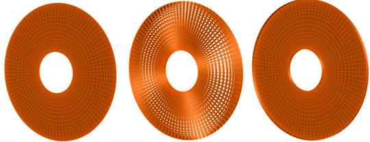
As shown in Figure 34.34: From Left to Right, the Three Components of the Disk Cell Zone: Int_Acdisk, Int_Disk and Int_Disk:003, Fluent automatically subdivides the disk cells into three separate entities:
int_acdisk contains the internal single-sided cell faces lying on the actuator disk surface.
int_disk:003 contains the cell faces shared by the live and disk domains, excluding the actuator disk.
int_disk contains the internal cell faces perpendicular to the disk.
To display the first two surfaces, select each in the list of Surfaces, and click .
For the third surface, however, click Adjacency in the Mesh Display dialog box to open the Adjacency dialog box, select disk from the list of Cell Zone(s) and int_disk from the list of the Adjacent Face Zones and then click the Display Face Zones.
Note: If this arrangement is not respected, the VBM will not work properly.
Figure 34.34: From Left to Right, the Three Components of the Disk Cell Zone: Int_Acdisk, Int_Disk and Int_Disk:003
Since this tutorial uses the Embedded Disk VBM Mode, the following mesh topology requirements must be respected:
The entire 360˚ azimuth of the propeller disk must be modeled.
The actuator disk surface (int_acdisk) must have the interior boundary condition.
The cells attached to one side of the disk must be marked as a separate domain (disk).
These cells must have one complete face attached to the disk. Only hexa and prisms are allowed.
A continuum fluid zone (live) must completely envelop the rotor zone (disk).
The fluid zone and rotor zone must have different BC index (10 for the fluid zone and 1 for the rotor zone).
Fluent VBM can be enabled through the VBM Rotor Inputs dialog box or through the Text User Interface (TUI) by using the following text user interface command in the Fluent Console:
define/models/virtual-blade-model/enable?
Answer yes when asked to enable the Virtual Blade Model.
Note: The VBM is only available with Dimension set to 3D.
The VBM can only be enabled when a valid Ansys Fluent case or mesh file has been set or read.
The current compatibility of the VBM is limited as it cannot operate with multiphase or inviscid flow. If any of these are active, Fluent will prevent the VBM from being enabled and display a warning message via either the Console or a pop-up message.
Since this tutorial is in the SI system of units, and the rotor disk, blade pitch and blade flapping angles are provided in degree, go to:
![]() Domain → Mesh
→ Units...
Domain → Mesh
→ Units...
Click the si tab.
Click angle in the Quantities list and choose in the Units list.
Close the Set Units dialog box.
To set the operating conditions, go to:
![]() Physics →
Physics →
Set a value of
97013.91Pascal in the Operating Pressure box.Set a value of
-1m in the X component of the Reference Pressure Location section.Click .
To configure the Fluent solver settings, go to:
Physics →
and select the following options in the General task page:
Type → Pressure-Based
Velocity Formulation → Absolute
Time → Steady
To enable the energy equation, go to:
Physics →
Models and enable the Energy equation box.
To select the turbulence model, go to:
Physics →
Models → Select the Spalart-Allmaras (1-eqn) turbulence model.
Enable the Strain/Vorticity-Based production option.
Enable Curvature Correction in the Options section.
Click to accept all the other default settings and close the Viscous Model dialog box.
For vorticity-dominated flows, the default Vorticity-Based-production option overpredicts the production of eddy viscosity in the vortex cores. Adding the strain tensor to the vorticity reduces the production of turbulent viscosity in regions where the measure of vorticity exceeds that of strain rate.
This simulation features a high-speed flow regime, hence compressibility must be enabled. Go to:
![]() Physics → Materials
→
Physics → Materials
→
Select air as the working fluid in the Fluid Materials pull-down menu.
Select ideal-gas in the Density pull-down menu.
Click the button.
Close the Create/Edit Materials dialog box.
Note: The VBM also works with the constant density and incompressible-ideal-gas options, however since rotors usually operate in the compressible regime, the ideal-gas option is more appropriate.
To configure the boundary conditions, go to:
![]() Physics → Zones
→ Boundaries
Physics → Zones
→ Boundaries
Set the boundary condition at the inlet.
Select the inflow boundary in the Task Page, ensure that its Type is velocity-inlet and click the button.
In the Momentum panel of the ribbon, select the Components option from the Velocity Specification Method pull-down menu.
Select Absolute in the Reference Frame pull-down menu.
Input the values (
84.54519,0,0) m/s for the X-, Y- and Z-Velocity components, respectively.In the Turbulence section, select the Turbulent Viscosity Ratio option from the Specification Method pull-down menu and set the Turbulent Viscosity Ratio to
1.In the Thermal panel of the ribbon, set a Temperature value of
284.5926K.Click and close the Velocity Inlet dialog box.
Set the boundary condition at the outlet.
Select the outflow boundary, ensure that the Type is pressure-outlet, then click the button.
Select Absolute in the Backflow Reference Frame pull-down menu.
Set the Gauge Pressure value to
0Pascal.In the Turbulence section, select the Modified Turbulent Viscosity option in the Specification Method pull-down menu.
Set a value of
0.0001(m2/s) in the Backflow Modified Turbulent Viscosity box.There is very little chance that backflow may occur, however it is good practice not to skip this operation.
In the Thermal panel of the ribbon, set the Backflow Total Temperature to
288.15K.Click and close the Pressure Outlet dialog box.
Set the Wall boundary conditions.
Select the Outer boundary and click on the button.
In the Momentum panel of the ribbon, set the Shear Condition to Specified Shear with {
0,0,0} X-, Y- and Z-Components, respectively, and click the button.In the Thermal panel of the ribbon, select Heat Flux in the Thermal Conditions and ensure that the Heat Flux value is
0W/m2.Click and close the Wall dialog box.
To set the reference values, go to:
![]() Physics → Reference
Values…
Physics → Reference
Values…
Select inflow from the Compute from pull-down menu.
Set the Area value to
0.785398m2 (disk area).Set the Length Value to
0.05m (the blade tip chord).Select live from the Reference Zone pull-down menu.
To set the discretization options, go to:
Solution → Solution
Methods… In the Solution Methods task page, use the pull-down menus to set the following options:
Scheme → Coupled
Gradient → Green-Gauss Node Based*
Pressure → PRESTO!**
Density → Second Order Upwind
Momentum → Second Order Upwind
Modified Turbulent Viscosity → First Order Upwind
Energy → Second Order Upwind
Pseudo Time Method →
Note: *The node-based averaging scheme is more accurate than the default cell-based scheme, especially for unstructured meshes, and most notably for triangular and tetrahedral meshes.
**The PRESTO! pressure discretization scheme is recommended for rotating flows.
Retain the default solver parameters in:
Solution →
Controls →
Controls...→ Solution
Controls..
Initialize the solution from inlet boundary values. Go to:
![]() Solution →
Initialization
Solution →
Initialization
Select Standard and click to open the Solution Initialization task page, which provides access to further settings.
Select from the Compute from drop-down list.
Set the Reference Frame to .
Click the button.
The last step before running the case is the configuration of the physical parameters of the propeller. To set up rotor parameter, go to:
![]() →
→
→
→
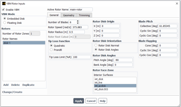
Select to open the VBM Rotor Inputs dialog box.
Ensure is enabled.
Select Embedded Disk as VBM Mode.
Press under Rotor Names list to add a new rotor. A new rotor with a default name disk-1 with default properties will be created. These entries will be updated in the next steps.
Enter
main-rotorin the Active Rotor Name box to change the rotor name.Enter the parameters shown in Figure 34.35: General Disk Data Configuration Window.
Click int_acdisk in the list of Surfaces to select the actuator disk surface.
Click the button of the ribbon and enter the parameters shown in Figure 34.36: Geometry Configuration Window.
Click to save the settings.
Click to close the VBM Rotor Inputs dialog box.
Note: The button must be clicked before moving on to the next rotor (when present) or before pressing the button. This sequence must always be respected, even if the VBM Rotor Inputs dialog box is re-opened to simply edit a parameter.
When pressing , Fluent VBM reads and pre-processes data entered in the VBM Rotor Inputs dialog box and reports information regarding each rotor zone.
The VBM will append the .dat suffix to the airfoil file names if it is omitted in the VBM graphical user interface.
Consult Airfoil File Format within the Fluent User's Guide for more information on the geometry of the rotor disk and the effect of the parameters.

To configure the residuals monitors that will appear in the Fluent graphics window and Console, go to:
Solution →
Reports →
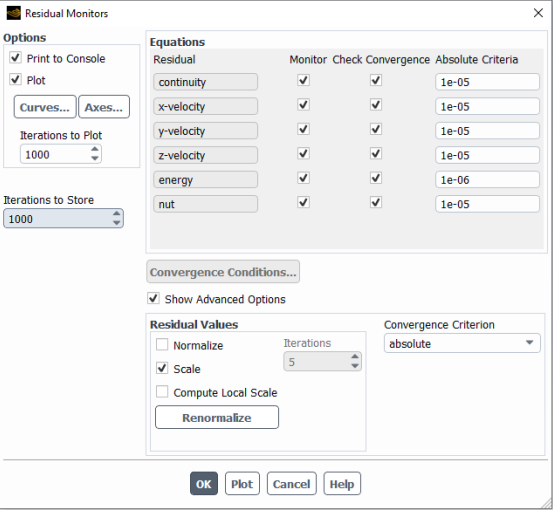
Ensure that and options are enabled in the Options group box.
Enable and select from the Convergence Criterion drop-down list.
Set the Absolute Criteria values to
1e-6for the energy equation and to1e-5for the other equations as shown in Figure 34.37: Solution Residuals Configuration.Click to close the Residual Monitors dialog box.
Additionally, you may want to monitor pressure convergence on the actuator disk int_acdisk. Go to:
Solution →
Reports →
→ → Surface
Report → Integral… Enter
rotor-pressurein the Name box.Enable Report File, Report Plot and Print to Console in the Create section.
Select Pressure… and Static Pressure with the pull-down menus in the Field Variable section.
Select int_acdisk in the Surfaces section.
Click to close the Surface Report Definition dialog box.
When the calculation begins, the pressure convergence history will be displayed on screen and written in the file rotor-pressure-rfile.out.
Additionally, the convergence histories of the thrust, torque, power, moments and forces are automatically written to the Rotor_1_Loads.dat file. If you want to see the convergence histories of any output quantity (for example, VBM Thrust) for the rotor, Go to:
Solution →
Reports → Definitions
→ →
→ Rotor Thrust…Enter
main-rotor-thrustin the Name box.Enable , and in the Create section.
Select under Report Type.
Select under Output Type.
Select main-rotor in the Rotor Names list.
Click to close the dialog box.
When the calculation begins, the rotor thrust convergence history will be displayed in the Graphics window, printed in the Console and written in main-rotor-thrust-rfile.out.
Example 34.2: The ribbon at the top of the Graphics window can be used to change the view options defined above.
(residual/pressure-integral/rotor-thrust convergence history)
It's recommended to set up and save the post-processing configuration before proceeding with the actual solution process. Nevertheless, if you prefer, you may skip this section and configure the post-processing setup later after obtaining the solution.
Create a cutting plane through the wake of the propeller to visualize the momentum changes produced by the actuator disk. The cutting plane will also enable a comparison of the effect of trimming on the solution. Go to:
![]() Results →
Surface → →
Results →
Surface → →
Enable Point and Normal in the Method list. This will allow the creation of an unbounded cutting plane.
Enter the name
plane-z=0in the New Surface Name box.Enter the coordinates of the origin of int_acdisk in the Point section: P(0) = {
0,0,0}Enter the components of the cutting plane Normal vector n = {
0,0,1}Click the button and close the Plane Surface dialog box
Create a cutting plane through the rotor zone, parallel to the disk, such that it cuts all prismatic elements in the rotor zone (disk). This cutting plane will be used to visualize the VBM data distributions on the disk. To create this plane, go to:
![]() Results →
Surface → →
Results →
Surface → →
Enter the name
disk-planein the New Surface Name box.Select and then from the Surface of Constant drop-down list.
Select disk in the From Zones list.
Set the Iso-Values to
0m.Click the button and close the Iso-Surface dialog.
The two simulations can now be executed to demonstrate the capabilities of the VBM. Before starting the simulation, it is a good idea to save the work at this point. Go to
![]() → →
→ →
and save the settings into the VBM_propeller_tutorial.cas file. Alternately, the option can be used.
For the first simulation, the propeller is operating in fixed-pitch mode without trimming. Go to:
Solution → Run Calculation → Run Calculation...
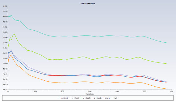
Set the No. of Iterations value to
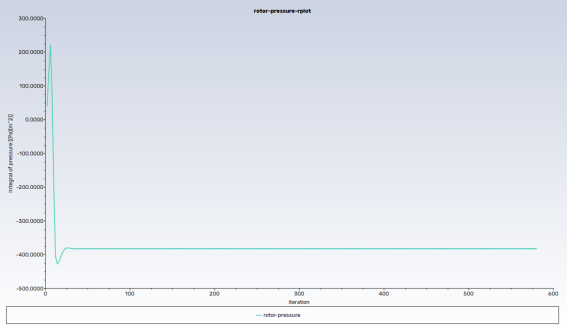
600and click the button. The convergence history of the residuals of the governing equations is shown in Figure 34.38: Convergence History with Fixed Pitch. Figure 34.39: Pressure Monitor Convergence History with Fixed Pitch shows the convergence history of the integral of the static pressure on the int_acdisk surface.Save the Fluent case and data files (VBM_propeller_tutorial_FP.cas and .dat):
→
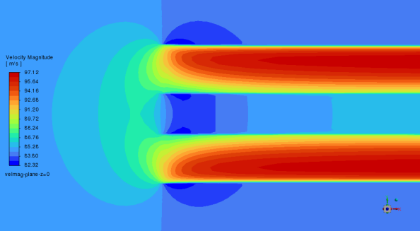
→ To display contours of flow velocity on the cutting plane that has been created in Cutting Plane for the Velocity Distributions, go to:
Results →
Graphics →
→ Configure the window as shown in Figure 34.41: Display the Velocity Distribution on the Z = 0 Cutting Plane.
Click the button to display the image in the graphics window.
Click the blue z-axis arrow in the axis triad and zoom in to see the velocity contours on plane-z=0 near the actuator disk, as shown in Figure 34.42: Velocity Magnitude Distribution Around the Actuator Disk, Z = 0 Cutting Plane.
To change the colormap, click to open the Colormap dialog and set the parameters (Number Format, Font Size, Colormap Size, etc) based on your preference.
Figure 34.42: Velocity Magnitude Distribution Around the Actuator Disk, Z = 0 Cutting Plane shows the flow contraction by the propeller in the downstream of the propeller. The axial velocity is increased from 84.5 to 97 at some regions.
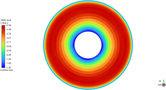
To display the VBM data like angle of attack on the disk, go to:
Results →
Graphics →
→ Ensure Node Value and Global Range are deselected in the Options group box.
Note: The VBM variables are cell-based, therefore the Node Value check box must be de-selected in order for the values to display correctly. Re-orient the viewing position along the positive x-axis.
Select disk-plane in the list of Surfaces, then select the VBM Model... and desired options from the pull-down menu.
Click the button.
The contours of Angle of Attack (AoA) are shown in Figure 34.43: Angle of Attack Distribution on the Actuator Disk. This is a useful visual verification that the angle of attack is within the active region of the aerodynamic properties of the airfoil section (see Problem Description). Figure 34.43: Angle of Attack Distribution on the Actuator Disk shows the radial distribution of the blade pitch angle.
The next simulation should yield identical results to the previous one, with the exception that now the VBM will trim the blade pitch angle (collective angle) of the propeller to match the same thrust. It is expected that the trimming will recover the exact blade pitch angle of the fixed-pitch propeller.
Before enabling the collective trimming, the thrust coefficient of the fixed-pitch propeller needs to be computed from the fixed-pitch solution with the following equation:

Table 34.6: Values From the Fixed-Pitch Solution lists the values of the
variables to insert in the formula. The rotor thrust  can be recovered from column 3 of the last line of the VBM log
file Rotor_1_Loads.csv.
can be recovered from column 3 of the last line of the VBM log
file Rotor_1_Loads.csv.
 is the coefficient of the dynamic pressure, set to
 1 in the code. The blade tip velocity and
the reference density are taken from Table 34.4: Propeller Geometric Data and Operating Conditions.
Note: The usage of tip speed rather than the customary propeller axial velocity.
Table 34.6: Values From the Fixed-Pitch Solution
| Variable | Value | |
|---|---|---|
 | rotor thrust | 761.9573 N |
 | dynamic pressure coefficient | 1 |
 | blade tip velocity | 186.9415 m/s |
 | reference density | 1.187584 kg/m3 |
 | rotor diameter | 1 m |
The computed thrust coefficient value CT is 0.02337572.
To enable collective trimming, go to:
Physics →
Models → Select the to open the VBM Rotor Inputs dialog box.
Set the Collective angle to
55˚.Click the button in the ribbon and enable Collective pitch.
Set the Update Frequency value to
10, the Damping Factor to0.7and enter0.02337572in the Desired thrust coefficient box.Click the button, then press .
To run the calculation, go to:
Solution → Run
Calculation → Run Calculation... Enter a value of
600in the No. of Iterations box and press the button.This run is intended to verify that the thrust coefficient value is precise and the collective angle printed to the Console after 600 iterations converges towards the original 61.85345-degrees fixed-pitch blade angle.
When the execution terminates, save the case and data files (VBM_propeller_tutorial_VP.cas and .dat):
→
→
At convergence the residual history and pressure monitor history will resemble Figure 34.44: Convergence History with Collective Trimming and Figure 34.45: Pressure Monitor Convergence History with Collective Trimming. The convergence history shown in Figure 34.46: Rotor Thrust Monitor Convergence History demonstrates the gradual increase of rotor thrust through the adjustment of collective pitch by the VBM trim routine.
The converged rotor thrust with collective trimming is listed in the third column of the Ro- tor_1_Loads.csv log file as 761.9573 N. At convergence, the collective angle reported on the Fluent Console is 61.853442, compared to the fixed-pitch setting of 61.85344°.
This simple tutorial shows that Fluent VBM, which was originally written for helicopter rotor simulations, can also be used to simulate propellers, even when the actuator disk, the propeller analogue, is not aligned with the natural helicopter rotor disk orientation (Z-axis).
Step-by-step instructions for the Fluent and VBM set-up are provided to enable you to conduct realistic propeller simulations.
The comparison of the fixed-pitch results with the collective trimming case implicitly demonstrates that the VBM trimming routine is stable and accurate.
Considering the coarseness of the grid, which has been tailored towards portability, simplicity and fast turnaround of the tutorial runs, rather than accuracy, very reasonable results have been obtained for both the fixed-pitch and collective trimming simulations.
Capitao Patrao, A., “Description and Validation of the rotorDiskSource Class for Propeller Performance Estimation,” In: Proceedings of CFD with OpenSource Software, 2017, Edited by Nilsson., H.
Glauert, H. “The Elements of Aerofoil and Airscrew Theory,” Second Edition, Cambridge University Press, New York, USA, 1947.
Stepniewski, W.Z. and Keys, C.N., “Rotary-Wing Aerodynamics,” Dover Publications Inc., New York, USA, 1984.
Leishman, J.G., “Principles of Helicopter Aerodynamics,” Cambridge University Press, New York, USA, 2000.
Zori, L.A.J., Rajagopalan, R.G., “Navier-Stokes Calculation of Rotor-Airframe Interaction in Forward Flight”, Journal of the American Helicopter Society, Vol.40, April 1995.